H. Rates Volatility Modeling: An Overview

import IPython; IPython.display.HTML('''<script>code_show=false; function code_toggle() { if (code_show){ $('div.nbinput').show(); } else { $('div.nbinput').hide(); } code_show = !code_show} $( document ).ready(code_toggle);</script><form action="javascript:code_toggle()"><input type="submit" value="Click here to toggle on/off the raw code."></form>''')

Agenda

Part I: Vanilla Models

• Option Pricing Basics, Binomial Tree

• Vanilla Option Pricing Models

  • SABR

  • Displaced Lognormal

• Change of Numeraire

• Applications

  • Swaption Pricing In SABR

  • CMS Spread Option Pricing With Copula

Part II: Term Structure Models

• HJM Framework, Forward Rate Vol

• Hull-White Model

• Cheyette

Option Pricing Basics

• The Fundamental Principle: In a no-arbitrage market, the price of any derivative with payoff \(X\) is the expectation of its discounted payoff under the risk-neutral measure \(P^M\)

• The Universal Formula:

  • \(M_t\): Time-\(t\) value of the money market account with \(M_0 = 1\) (the numeraire)

  • \(P^M\): The risk-neutral probability measure associated with \(M\)

    \[V_0 = M_0 E^M \left[ M_T^{-1} X_T \right]\]

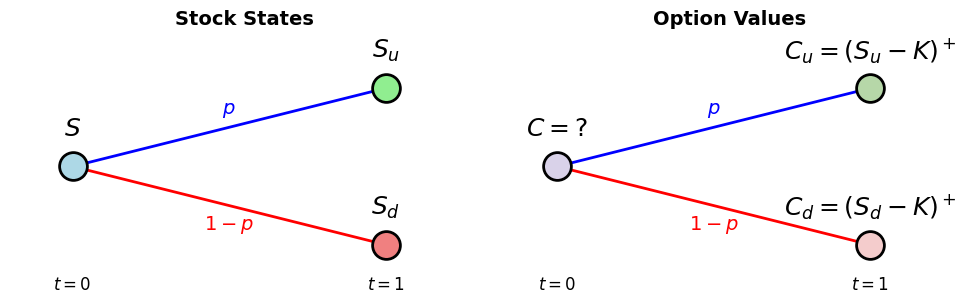
Binomial Option Pricing Model (BOPM)

• We want to price an option on a stock trading at \(S\) currently

• Assumptions:

  • Only two discrete times (one time step): Today at \(t=0\) and maturity at \(t=1\)

  • At \(t=1\), the stock price can either go up to \(S_u\) or go down to \(S_d\) (two states), with corresponding option prices \(C_u\) and \(C_d\), respectively

  • A money market account (MMA) with initial value 1 will become \(M\) at \(t=1\)

# Single-step binomial tree visualization (stock + option payoff tree)
import matplotlib.pyplot as plt

fig, (ax_stock, ax_opt) = plt.subplots(1, 2, figsize=(10, 3.5))

# Shared node positions
t0_x, t0_y = 0, 0.5
t1_u_x, t1_u_y = 1, 0.75
t1_d_x, t1_d_y = 1, 0.25
node_size = 400

# -------- Left panel: stock tree --------
ax_stock.plot([t0_x, t1_u_x], [t0_y, t1_u_y], 'b-', lw=2, label='Up move')
ax_stock.plot([t0_x, t1_d_x], [t0_y, t1_d_y], 'r-', lw=2, label='Down move')
ax_stock.scatter([t0_x], [t0_y], s=node_size, c='lightblue', edgecolors='black', zorder=5, linewidths=2)
ax_stock.scatter([t1_u_x], [t1_u_y], s=node_size, c='lightgreen', edgecolors='black', zorder=5, linewidths=2)
ax_stock.scatter([t1_d_x], [t1_d_y], s=node_size, c='lightcoral', edgecolors='black', zorder=5, linewidths=2)
ax_stock.text(t0_x, t0_y + 0.12, r'$S$', fontsize=18, ha='center', va='center', fontweight='bold')
ax_stock.text(t1_u_x, t1_u_y + 0.12, r'$S_u$', fontsize=18, ha='center', va='center', fontweight='bold')
ax_stock.text(t1_d_x, t1_d_y + 0.12, r'$S_d$', fontsize=18, ha='center', va='center', fontweight='bold')
ax_stock.text(0.5, 0.65, r'$p$', fontsize=14, ha='center', va='bottom', color='blue')
ax_stock.text(0.5, 0.35, r'$1-p$', fontsize=14, ha='center', va='top', color='red')
ax_stock.text(t0_x, 0.15, r'$t=0$', fontsize=12, ha='center', va='top')
ax_stock.text(t1_u_x, 0.15, r'$t=1$', fontsize=12, ha='center', va='top')
ax_stock.set_xlim(-0.2, 1.3)
ax_stock.set_ylim(0.2, 0.9)
ax_stock.set_aspect('equal')
ax_stock.axis('off')
ax_stock.set_title('Stock States', fontsize=14, fontweight='bold', pad=12)

# -------- Right panel: option value tree --------
ax_opt.plot([t0_x, t1_u_x], [t0_y, t1_u_y], 'b-', lw=2)
ax_opt.plot([t0_x, t1_d_x], [t0_y, t1_d_y], 'r-', lw=2)
ax_opt.scatter([t0_x], [t0_y], s=node_size, c='#d9d2e9', edgecolors='black', zorder=5, linewidths=2)
ax_opt.scatter([t1_u_x], [t1_u_y], s=node_size, c='#b6d7a8', edgecolors='black', zorder=5, linewidths=2)
ax_opt.scatter([t1_d_x], [t1_d_y], s=node_size, c='#f4cccc', edgecolors='black', zorder=5, linewidths=2)
ax_opt.text(t0_x, t0_y + 0.12, r'$C=?$', fontsize=18, ha='center', va='center', fontweight='bold')
ax_opt.text(t1_u_x, t1_u_y + 0.12, r'$C_u = (S_u - K)^+$', fontsize=18, ha='center', va='center', fontweight='bold')
ax_opt.text(t1_d_x, t1_d_y + 0.12, r'$C_d = (S_d - K)^+$', fontsize=18, ha='center', va='center', fontweight='bold')
ax_opt.text(0.5, 0.65, r'$p$', fontsize=14, ha='center', va='bottom', color='blue')
ax_opt.text(0.5, 0.35, r'$1-p$', fontsize=14, ha='center', va='top', color='red')
ax_opt.text(t0_x, 0.15, r'$t=0$', fontsize=12, ha='center', va='top')
ax_opt.text(t1_u_x, 0.15, r'$t=1$', fontsize=12, ha='center', va='top')
ax_opt.set_xlim(-0.2, 1.3)
ax_opt.set_ylim(0.2, 0.9)
ax_opt.set_aspect('equal')
ax_opt.axis('off')
ax_opt.set_title('Option Values', fontsize=14, fontweight='bold', pad=12)

# fig.suptitle('One-Step Binomial Trees', fontsize=16, fontweight='bold', y=1.02)
plt.tight_layout()
plt.show()

BOPM No-Arbitrage Argument

• Replication Argument:

  • Set up a portfolio so that its value at \(t=1\) replicates the option in both states

  • By no-arbitrage, the option price and the portfolio value at \(t=0\) should equal

• The portfolio setup at \(t=0\):

  • Buy \(\Delta {\color{lightgray}~= (C_u - C_d)/(S_u - S_d)}\) shares of the stock at \(S\)

  • Deposit \(B {\color{lightgray}~= (C_dS_u - C_uS_d)/(M(S_u - S_d))}\) dollars into MMA

• It can be easily verified that the portfolio value and option price agree at \(t=1\) in both states: \begin{align*} \Delta S_u + BM &= C_u\\ \Delta S_d + BM &= C_d \end{align*}

• Initial portfolio value is \(\Delta S+B\):

  \[C = \underbrace{\color{lightgray}\left(\frac{SM - S_d}{S_u - S_d}\right)}_{p^M} \frac{C_u}{M} + \underbrace{\color{lightgray}\left(\frac{S_u - SM}{S_u - S_d}\right)}_{1-p^M} \frac{C_d}{M} = M_0E^M[M^{-1}_T X]\]

Risk-Neutral Probability in BOPM

• \(p^M \ne p\) the physical probability which is not in the story

• Even if an agent is confident about \(p\), he/she should still quote the option at the fair price \(M_0E^M[M_T^{-1} X]\), as that’s the price to guarantee no arbitrage

Delta Hedge in BOPM

• Replicating Portfolio

  • \(\Delta = (C_u - C_d)/(S_u - S_d)\) shares of the stock at \(S\)

  • Some MMA (risk free)

\begin{align*} \text{Option} &= \text{Replicating Portfolio}\\ &= \Delta\text{ Shares of Stock} + \text{MMA} \end{align*}

\[\text{Option} - \Delta\text{ Shares of Stock} = \text{MMA}\]

Multi-Step BOPM

• Pricing: Construct replicating portfolios at each one-step sub-tree, computing expectations under the risk-neutral probability backward in time from maturity \(T\)

• Dynamic Hedging: Compute \(\Delta\) at each node and dynamically rebalance to ensure a locally risk-free portfolio across every time step

# 3-step recombining binomial tree visualization
import matplotlib.pyplot as plt

fig, ax = plt.subplots(figsize=(5, 2.5))

steps = 3
node_size = 400

# Draw recombining tree nodes and edges
for i in range(steps):
    for j in range(i + 1):
        # Current node (t=i)
        curr_x = i
        curr_y = j * 2 - i

        # Up move (t=i+1)
        up_x = i + 1
        up_y = (j + 1) * 2 - (i + 1)
        ax.plot([curr_x, up_x], [curr_y, up_y], 'b-', lw=1.5, alpha=0.6)

        # Down move (t=i+1)
        down_x = i + 1
        down_y = j * 2 - (i + 1)
        ax.plot([curr_x, down_x], [curr_y, down_y], 'r-', lw=1.5, alpha=0.6)

# Scatter plot for nodes to overlay on top of lines
for i in range(steps + 1):
    for j in range(i + 1):
        x = i
        y = j * 2 - i
        ax.scatter(x, y, s=node_size, c='lightblue', edgecolors='black', zorder=5, linewidths=1.5)
        # Label each node generically, or using S_... string
        # Number of up moves = j, number of down moves = i - j
        # ax.text(x, y, f'{j}U\n{i-j}D', fontsize=9, ha='center', va='center', fontweight='bold', zorder=10)

ax.set_xticks(range(steps + 1))
ax.set_xticklabels([f't={i}' for i in range(steps + 1)])
ax.set_yticks([])
ax.set_xlim(-0.5, steps + 0.5)
ax.set_ylim(-steps - 0.5, steps + 0.5)
ax.axis('off')

# Explicitly add time labels at the bottom since axis is off
for i in range(steps):
    ax.text(i, -steps - 0.8, f'$t=${i}', fontsize=12, ha='center', va='top')

ax.text(steps, -steps - 0.8, f'$t=T$', fontsize=12, ha='center', va='top')

# ax.set_title('3-Step Recombining Binomial Tree', fontsize=14, fontweight='bold', pad=15)

plt.tight_layout()
plt.show()

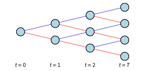
• With infinitely many time steps, the tree describes a continuous-time stochastic process, and with right assumptions the option price converges to the Black-Scholes formula

Vanilla Option Pricing Models

• All we need is a terminal distribution at the expiry \(T\) if our goal is to price/hedge one single vanilla option

• Black Normal Model: The underlying (say, a forward rate) follows a scaled Brownian motion

  \[dF_t = \sigma\,dW_t \quad\implies\quad F_T\sim N(0, \sigma^2 T),\]

  which leads to nice closed form formulas

• The Reality: Rates are not normally distributed. The market implied distribution has nonzero skewness and excess kurtosis

  • We need models, like SABR, that parameterize the first 4 moments of the distribution

• Implied Volatility: Equating the Black normal formula and the market/model price and back out \(\sigma\)

SABR

• \(\alpha\) controls overall level of the implied vol (2nd moment of the distribution)

• \(\rho\) controls the implied vol skew (skewness of the distribution, the 3nd moment)

• \(\nu\) (vol of vol) controls the implied vol convexity (kurtosis, the 4th moment) \begin{align*} \begin{cases} dF_t = \alpha_tF_t^{\beta}\,dW_t\\ d\alpha_t = {\color{red}\nu} \alpha_t\,dZ_t, \qquad {\color{red}\alpha_0 = \alpha}\\ dW_tdZ_t = {\color{red}\rho} dt \end{cases} \end{align*}

SABR (Cont.)

• \(\alpha\) controls overall level of the implied vol (2nd moment of the distribution)

• \(\rho\) controls the implied vol skew (skewness of the distribution, the 3nd moment)

• \(\nu\) (vol of vol) controls the implied vol convexity (kurtosis, the 4th moment)

import numpy as np

def _f_minus_k_ratio(f, k, beta):
    """Hagan's 2002 f minus k ratio - formula (B.67a)."""
    eps = 1e-07  # Numerical tolerance for f-k and beta
    if abs(f-k) > eps:
        if abs(1-beta) > eps:
            return (1 - beta) * (f - k) / (f**(1-beta) - k**(1-beta))
        else:
            return (f - k) / np.log(f / k)
    else:
        return k**beta


def _zeta_over_x_of_zeta(k, f, t, alpha, beta, rho, volvol):
    """Hagan's 2002 zeta / x(zeta) function - formulas (B.67a)-(B.67b)."""
    eps = 1e-07  # Numerical tolerance for zeta
    f_av = np.sqrt(f * k)
    zeta = volvol * (f - k) / (alpha * f_av**beta)
    if abs(zeta) > eps:
        return zeta / _x(rho, zeta)
    else:
        # The ratio converges to 1 when zeta approaches 0
        return 1.


def _x(rho, z):
    """Hagan's 2002 x function - formula (B.67b)."""
    a = (1 - 2*rho*z + z**2)**.5 + z - rho
    b = 1 - rho
    return np.log(a / b)


def normal_vol(k, f, t, alpha, beta, rho, volvol):
    """Hagan's 2002 SABR normal vol expansion - formula (B.67a)."""
    # We break down the complex formula into simpler sub-components
    f_av = np.sqrt(f * k)
    A = - beta * (2 - beta) * alpha**2 / (24 * f_av**(2 - 2 * beta))
    B = rho * alpha * volvol * beta / (4 * f_av**(1 - beta))
    C = (2 - 3 * rho**2) * volvol**2 / 24
    FMKR = _f_minus_k_ratio(f, k, beta)
    ZXZ = _zeta_over_x_of_zeta(k, f, t, alpha, beta, rho, volvol)
    # Aggregate all components into actual formula (B.67a)
    v_n = alpha * FMKR * ZXZ * (1 + (A + B + C) * t)
    return v_n

import numpy as np
import matplotlib.pyplot as plt
from scipy.stats import norm
from pandas import DataFrame
from ipywidgets import interact

import warnings
warnings.filterwarnings('ignore')

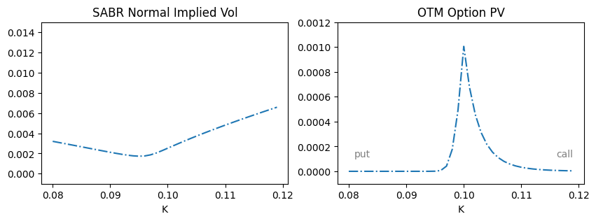
@interact(alpha=(0.001, 0.01, 0.001), rho=(-0.99, 0.99, 0.1), volvol=(0.01, 1, 0.1))
def plot(alpha=0.01, rho=0., volvol=0.6):
    beta = 0.6
    F = 0.1
    T = 1
    a = 0.08
    b = 0.12

    fig, (ax1, ax2) = plt.subplots(1, 2, figsize=(10, 3))
    def call(K, F, T, A=1):
        iv = normal_vol(K, F, T, alpha, beta, rho, volvol)
        d = (F-K)/(iv*np.sqrt(T))
        return A*iv*np.sqrt(T)*(norm.pdf(d) + d*norm.cdf(d))

    def put(K, F, T, A=1):
        return call(K, F, T, A) + A*(K-F)

    DataFrame([(K, normal_vol(K, F, T, alpha, beta, rho, volvol)) for K in np.arange(a, b, 0.001)], columns=['K', 'Implied Vol']).set_index('K').plot(style='-.', legend=None, ax=ax1)
    ax1.set(ylim=(-0.001, 0.015), title='SABR Normal Implied Vol')

    DataFrame([(K, call(K, F, T) if K>F else put(K, F, T)) for K in np.arange(a, b, 0.001)], columns=['K', 'OTM Options']).set_index('K').plot(style='-.', legend=None, ax=ax2)
    ax2.set(ylim=(-0.0001, 0.0012), title='OTM Option PV')
    ax2.text(a + 0.001, 0.0001, 'put', fontsize=10, ha='left', va='bottom', color='gray')
    ax2.text(b - 0.001, 0.0001, 'call', fontsize=10, ha='right', va='bottom', color='gray')
    plt.show()

SABR \(\rho\): The Intuition

• Why does \(\rho\), the rates vol correlation, control the IV skew?

  • Consider an OTM call and put at the same absolute moneyness. They are only trading positive because they might become ITM as the underlying moves

  • When \(\rho \gg 0\) (and vice versa for \(\rho \ll 0\))

    • Upside Move: Call becomes ITM, the vol increases

    • Downside Move: Put becomes ITM, the vol decreases

    • As option value increases with vol, the call is trading higher than the put

def plot_static(alpha=0.01, rho=0., volvol=0.6, figusize=(10, 3)):
    beta = 0.6
    F = 0.1
    T = 1
    a = 0.08
    b = 0.12

    fig, (ax1, ax2) = plt.subplots(1, 2, figsize=figusize)
    def call(K, F, T, A=1):
        iv = normal_vol(K, F, T, alpha, beta, rho, volvol)
        d = (F-K)/(iv*np.sqrt(T))
        return A*iv*np.sqrt(T)*(norm.pdf(d) + d*norm.cdf(d))

    def put(K, F, T, A=1):
        return call(K, F, T, A) + A*(K-F)

    DataFrame([(K, normal_vol(K, F, T, alpha, beta, rho, volvol)) for K in np.arange(a, b, 0.001)], columns=['K', 'Implied Vol']).set_index('K').plot(style='-.', legend=None, ax=ax1)
    ax1.set(ylim=(-0.001, 0.015), title='SABR Normal Implied Vol')

    DataFrame([(K, call(K, F, T) if K>F else put(K, F, T)) for K in np.arange(a, b, 0.001)], columns=['K', 'OTM Options']).set_index('K').plot(style='-.', legend=None, ax=ax2)
    ax2.set(ylim=(-0.0001, 0.0012), title='OTM Option PV')
    ax2.text(a + 0.001, 0.0001, 'put', fontsize=10, ha='left', va='bottom', color='gray')
    ax2.text(b - 0.001, 0.0001, 'call', fontsize=10, ha='right', va='bottom', color='gray')
    plt.show()

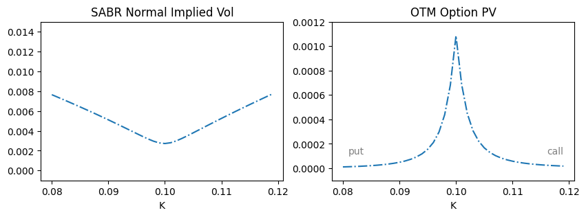
plot_static(rho=0.8)

SABR \(\nu\): The Intuition

• The Asymmetric Impact of \(\nu\) (vol of vol) Shocks

  • Deep (20%) OTM: Requires a vol spike to expire ITM; highly dependent on \(\nu\)

  • Near-the-Money (1% OTM): Insensitive to \(\nu\); outcome depends on today’s \(\alpha\)

• Results

  • As \(\nu\) goes up, distant tails become more expensive relative to the center

  • \(\nu\) as the “tail driver”, controls the probability of extreme volatility regimes

plot_static(volvol=1, figusize=(10, 3))

Displaced Lognormal Model

• An alternative way to parameterize the first 4 moments

• Volatility is a linear function of the underlying

  \[dF_t = (a_0 + {\color{red}a_1} F_t)\,dW_t\]

• \({\color{red}a_1}\) controls the IV skew, same as SABR’s \(\rho\):

  • When \(a_1 > 0\), the vol goes up as the underlying, same as the \(\rho \gg 0\) case (and vice versa for \(a_1 < 0\))

• Approximation of the general local volatility model \(dF_t = \sigma(F_t)\,dW_t\) as you can expand \(\sigma(\cdot)\)

• Has closed form formulas for NPV and Greeks

• Allows negative rates which lognormal does not

• Extension to SV gives us a vol of vol parameter \({\color{dodgerblue}\nu}\) to control the convexity of IV, while still preserving semi-closed form formulas

  \[\begin{split}\begin{align*} \begin{cases} \color{lightgray}dF_t = {\color{black}\alpha_t}(a_0 + a_1F_t)\,dW_t\\ d\alpha_t = k(\theta - \alpha_t)\,dt + {\color{dodgerblue}\nu}\sqrt{\alpha_t}\,dZ_t \end{cases} \end{align*}\end{split}\]

A Better Parametrization

• The displaced lognormal model can be parameterized as

  \[dF_t = \sigma( b F_t + (1-b) F_0)\,dW_t\]

• Why This Is Better:

  • For small \(t\) and vol, \(b F_t + (1-b) F_0 \approx F_0\) so \(\sigma\) has the same scale for all values of \(b\)

• Parameter Decoupling:

  • When \(\sigma\) changes, only the IV level changes, not the skew

  • When \(b\) changes, only the IV skew change, not the level

• Extension to SV:

  • \(\sigma\) can be made a stochastic volatility process, giving us a vol of vol parameter to control the convexity of IV, while still preserving semi-closed form formulas

Change of Numeraire

• Numeraire: A benchmark asset used as the denominator to price all other assets

• Change of Numeraire Formula:

  • \(N_t\): Time-\(t\) value of the Numeraire

  • \(P^N\): The probability measure associated with \(N\)

    \[V_0 = M_0 E^M \left[ M_T^{-1} X_T \right] = N_0 E^N \left[ N_T^{-1} X_T \right]\]

BOPM With Numeraire Asset

# Single-step binomial tree visualization (stock + option payoff tree)
import matplotlib.pyplot as plt

fig, (ax_stock, ax_opt) = plt.subplots(1, 2, figsize=(10, 3.5))

# Shared node positions
t0_x, t0_y = 0, 0.5
t1_u_x, t1_u_y = 1, 0.75
t1_d_x, t1_d_y = 1, 0.25
node_size = 400

# -------- Left panel: stock tree --------
ax_stock.plot([t0_x, t1_u_x], [t0_y, t1_u_y], 'b-', lw=2, label='Up move')
ax_stock.plot([t0_x, t1_d_x], [t0_y, t1_d_y], 'r-', lw=2, label='Down move')
ax_stock.scatter([t0_x], [t0_y], s=node_size, c='lightblue', edgecolors='black', zorder=5, linewidths=2)
ax_stock.scatter([t1_u_x], [t1_u_y], s=node_size, c='lightgreen', edgecolors='black', zorder=5, linewidths=2)
ax_stock.scatter([t1_d_x], [t1_d_y], s=node_size, c='lightcoral', edgecolors='black', zorder=5, linewidths=2)
ax_stock.text(t0_x, t0_y + 0.12, r'$S$', fontsize=18, ha='center', va='center', fontweight='bold')
ax_stock.text(t1_u_x, t1_u_y + 0.12, r'$S_u$', fontsize=18, ha='center', va='center', fontweight='bold')
ax_stock.text(t1_d_x, t1_d_y + 0.12, r'$S_d$', fontsize=18, ha='center', va='center', fontweight='bold')
ax_stock.text(0.5, 0.65, r'$p$', fontsize=14, ha='center', va='bottom', color='blue')
ax_stock.text(0.5, 0.35, r'$1-p$', fontsize=14, ha='center', va='top', color='red')
ax_stock.text(t0_x, 0.15, r'$t=0$', fontsize=12, ha='center', va='top')
ax_stock.text(t1_u_x, 0.15, r'$t=1$', fontsize=12, ha='center', va='top')
ax_stock.set_xlim(-0.2, 1.3)
ax_stock.set_ylim(0.2, 0.9)
ax_stock.set_aspect('equal')
ax_stock.axis('off')
ax_stock.set_title('Stock States', fontsize=14, fontweight='bold', pad=12)

# -------- Right panel: option value tree --------
ax_opt.plot([t0_x, t1_u_x], [t0_y, t1_u_y], 'b-', lw=2)
ax_opt.plot([t0_x, t1_d_x], [t0_y, t1_d_y], 'r-', lw=2)
ax_opt.scatter([t0_x], [t0_y], s=node_size, c='#d9d2e9', edgecolors='black', zorder=5, linewidths=2)
ax_opt.scatter([t1_u_x], [t1_u_y], s=node_size, c='#b6d7a8', edgecolors='black', zorder=5, linewidths=2)
ax_opt.scatter([t1_d_x], [t1_d_y], s=node_size, c='#f4cccc', edgecolors='black', zorder=5, linewidths=2)
ax_opt.text(t0_x, t0_y + 0.12, r'$N$', fontsize=18, ha='center', va='center', fontweight='bold')
ax_opt.text(t1_u_x, t1_u_y + 0.12, r'$N_u$', fontsize=18, ha='center', va='center', fontweight='bold')
ax_opt.text(t1_d_x, t1_d_y + 0.12, r'$N_d$', fontsize=18, ha='center', va='center', fontweight='bold')
ax_opt.text(0.5, 0.65, r'$p$', fontsize=14, ha='center', va='bottom', color='blue')
ax_opt.text(0.5, 0.35, r'$1-p$', fontsize=14, ha='center', va='top', color='red')
ax_opt.text(t0_x, 0.15, r'$t=0$', fontsize=12, ha='center', va='top')
ax_opt.text(t1_u_x, 0.15, r'$t=1$', fontsize=12, ha='center', va='top')
ax_opt.set_xlim(-0.2, 1.3)
ax_opt.set_ylim(0.2, 0.9)
ax_opt.set_aspect('equal')
ax_opt.axis('off')
ax_opt.set_title('Numeraire Asset Values', fontsize=14, fontweight='bold', pad=12)

# fig.suptitle('One-Step Binomial Trees', fontsize=16, fontweight='bold', y=1.02)
plt.tight_layout()
plt.show()

BOPM With Numeraire Asset (Cont.)

• If the MMA is replaced by a numeraire asset, the portfolio set up at \(t=0\):

  • Hold \(h\) share of the stock at \(S\)

  • Hold \(k\) units of the numeraire asset at \(N\)

• Equate the portfolio value and option price at \(t=1\) in both states: \begin{align*} hS_u + kN_u &= C_u\\ hS_d + kN_d &= C_d \end{align*}

• Initial portfolio value is \(h S + k N\):

  \[C = N\left[\underbrace{\color{lightgray}\left(\frac{SN_uN_d - S_dNN_u}{S_u NN_d - S_d NN_u}\right)}_{p^N} \frac{C_u}{N_u} + \underbrace{\color{lightgray}\left(\frac{-SN_uN_d + S_uNN_d}{S_u NN_d - S_d NN_u}\right)}_{1-p^N} \frac{C_d}{N_d} \right] = N_0E^N[N_T^{-1} X]\]

Swaption Pricing

def plot_swaption_timeline():

    import numpy as np
    import matplotlib.pyplot as plt

    fig, ax = plt.subplots(figsize=(11, 2.5))

    # Timeline coordinates
    x_t = 0.0
    timeline_x = [3.0, 4.0, 5.0, 6.0, 8.0]  # T0, T1, T2, T3, TN
    labels = [r"$T = T_0$", r"$T_1$", r"$T_2$", r"$T_3$", r"$T_N$"]

    # Draw main timeline with arrowhead at the end
    ax.annotate("", xy=(8.7, 0), xytext=(-0.4, 0),
                arrowprops=dict(arrowstyle="->", color="black", lw=2))
    ax.text(8.75, 0.12, r"$t$", ha="left", va="center", fontsize=14)

    # Mark today 0
    ax.vlines(x_t, -0.12, 0.12, color="black", linewidth=2)
    ax.text(x_t, -0.22, r"$0$", ha="center", va="top", fontsize=14)

    # Helper to draw a wiggly (floating-leg) arrow
    def draw_wiggly_arrow(ax, x, y0=0.05, y1=0.65, amp=0.05, waves=3.5, color="#1f77b4", lw=2):
        y = np.linspace(y0, y1, 180)
        phase = 2 * np.pi * waves * (y - y0) / (y1 - y0)
        taper = np.linspace(1.0, 0.0, y.size)
        x_wave = x + amp * np.sin(phase) * taper
        ax.plot(x_wave, y, color=color, linewidth=lw)
        ax.annotate(
            "",
            xy=(x, y1),
            xytext=(x, y1 - 0.08),
            arrowprops=dict(arrowstyle="->", color=color, lw=lw),
        )

    # Draw all timeline marks and labels
    for x, lab in zip(timeline_x, labels):
        ax.vlines(x, -0.12, 0.12, color="black", linewidth=2)
        ax.text(x, -0.22, lab, ha="center", va="top", fontsize=14)

    # Add accrual fractions between T0-T1, T1-T2, T2-T3
    tau_midpoints = [3.5, 4.5, 5.5]
    tau_labels = [r"$\tau_0$", r"$\tau_1$", r"$\tau_2$"]
    for x_tau, tau_lab in zip(tau_midpoints, tau_labels):
        ax.text(x_tau, 0.16, tau_lab, ha="center", va="center", fontsize=13, color="dimgray")

    # No payments at T0; payments start from T1
    payment_dates = timeline_x[1:]
    for x in payment_dates:
        draw_wiggly_arrow(ax, x)
        ax.annotate(
            "",
            xy=(x, -0.65),
            xytext=(x, -0.05),
            arrowprops=dict(arrowstyle="->", color="#d62728", lw=2),
        )

    # Show omitted intermediate payment dates between T3 and TN
    ax.text(7.0, 0.40, r"$\cdots$", color="#1f77b4", fontsize=20, ha="center", va="center")
    ax.text(7.0, -0.40, r"$\cdots$", color="#d62728", fontsize=20, ha="center", va="center")

    # Legend-like labels
    ax.text(8.35, 0.80, "Floating leg", color="#1f77b4", ha="right", fontsize=12)
    ax.text(8.35, -0.80, "Fixed leg", color="#d62728", ha="right", fontsize=12)

    ax.set_xlim(-0.4, 8.8)
    ax.set_ylim(-1.15, 1.15)
    ax.axis("off")
    # ax.set_title("Swaption Cashflow Timeline", fontsize=16, pad=10)

    plt.show()

plot_swaption_timeline()

\begin{align*} \text{Time-$t$ Forward Swap NPV} &= \sum_{n=0}^{N-1}\tau_n P(t, T_{n+1})({\color{darkcyan}L(t, T_n, T_{n+1}) \color{red}- K})\\ &= \underbrace{\left(\sum_{n=0}^{N-1}\tau_n P(t, T_{n+1})\right)}_{A(t)}\left(\underbrace{\frac{\sum_{n=0}^{N-1}\tau_n P(t, T_{n+1})L(t, T_n, T_{n+1})}{\sum_{n=0}^{N-1}\tau_n P(t, T_{n+1})}}_{S(t)}- K\right) \end{align*}

Swaption Pricing (Cont.)

• Step 1: Change numeraire to the annuity \begin{align*} \text{Payer Swaption NPV } &= M_0E^M[M_T^{-1} {\color{lightgray}(A_T (S_T - K))^+}]\\ &= A_0E^A[A_T^{-1} {\color{lightgray}(A_T (S_T - K))^+}]\\ &= A_0E^A[(S_T - K)^+] \end{align*}

• Step 2: Make assumption about \(S_t\) dynamics under the annuity measure, say to follow SABR \begin{align*} \begin{cases} dS_t = \alpha_tS_t^{\beta}\,dW_t^A\\ d\alpha_t = \nu \alpha_t\,dZ_t^A, \qquad \alpha_0 = \alpha\\ dW_t^AdZ_t^A = \rho dt \end{cases} \end{align*} The assumption only gives us \(E^A[(S_T - K)^+]\). We still need to get \(A_0\) from today’s curve

CMS Spread Option Pricing

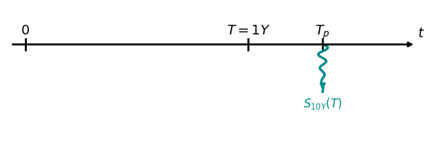
def plot_cms_timeline(cashflow_text=r"$(S_{\text{10Y}}(T) - S_{\text{2Y}}(T) - K)^+$", T_text=r"$T$", direction=1, figsize=(8, 2.5)):
    import matplotlib.pyplot as plt

    fig, ax = plt.subplots(figsize=figsize)

    # Time axis
    min_t, max_t = 0, 10

    # Draw main timeline with arrowhead at the end
    ax.annotate("", xy=(max_t + 0.5, 0), xytext=(-0.4, 0),
                arrowprops=dict(arrowstyle="->", color="black", lw=2))
    ax.text(max_t + 0.55, 0.12, r"$t$", ha="left", va="center", fontsize=14)

    # Markers for t=0, T, T_p
    T_val = 6
    T_p = 8

    ax.vlines(0, -0.07, 0.07, color="black", linewidth=2)
    ax.text(0, direction*(-0.22), "$0$", ha='center', va="top", fontsize=14)

    ax.vlines(T_val, -0.07, 0.07, color="black", linewidth=2)
    ax.text(T_val, direction*(-0.22), T_text, ha='center', va="top", fontsize=14)

    ax.vlines(T_p, -0.07, 0.07, color="black", linewidth=2)
    ax.text(T_p, direction*(-0.22), "$T_p$", ha='center', va="top", fontsize=14)

    # Helper to draw a wiggly (floating-leg) arrow
    def draw_wiggly_arrow(ax, x, y0=0.0, y1=0.5, amp=0.15, waves=3.5, color="darkcyan", lw=2.5):
        import numpy as np
        y = np.linspace(y0, y1, 180)
        phase = 2 * np.pi * waves * (y - y0) / (y1 - y0)
        taper = np.linspace(1.0, 0.0, y.size)
        x_wave = x + amp * np.sin(phase) * taper
        ax.plot(x_wave, y, color=color, linewidth=lw)
        ax.annotate(
            "",
            xy=(x, y1),
            xytext=(x, y1 - np.sign(y1 - y0) * 0.08),
            arrowprops=dict(arrowstyle="->", color=color, lw=lw),
        )

    # Drawing the cashflow
    cashflow_y = direction * 0.5
    draw_wiggly_arrow(ax, T_p, y0=0, y1=cashflow_y, amp=0.15, waves=3.5, color="darkcyan", lw=2.5)

    ax.text(T_p, cashflow_y + direction * 0.2, cashflow_text,
            ha='center', va='bottom', fontsize=12, color="darkcyan")

    if direction == 1:
        ax.set_ylim(-0.4, 1)
    else:
        ax.set_ylim(-1, 0.4)
    ax.set_xlim(-0.5, max_t + 1)
    ax.axis("off")

    plt.show()

plot_cms_timeline()

• All we need is a distribution \(\color{red}f_{S_{\text{10Y}}, S_{\text{2Y}}}(s_1, s_2)\): \begin{align*} \text{Cash Flow NPV} &= P(0, T_p) E^{T_p}[(S_{\text{10Y}}(T) - S_{\text{2Y}}(T) - K)^+]\\ &= P(0, T_p) \int\int(s_1 - s_2 - K)^+ {\color{red}f_{S_{\text{10Y}}, S_{\text{2Y}}}(s_1, s_2)}\,ds_1ds_2 \end{align*}

• If the joint distribution is known in closed form, NPV can be found by numerical integration

Delta Hedging CMS Spread Option

• Once we can find NPV \(V\), the spread Delta is the directional derivative of \(V\) along \(\vec u = \frac{1}{\sqrt{2}}(1, -1)\):

  \[\frac{\partial V}{\partial (S_1 - S_2)} = \nabla V \cdot u = \frac{\Delta_1 - \Delta_2}{\sqrt{2}},\]

  where the gradient is

  \[\nabla V = \left( \frac{\partial V}{\partial S_1}, \frac{\partial V}{\partial S_2} \right) = (\Delta_1, \Delta_2),\]

  the single rate Deltas

Copula

• While \(f_{S_{\text{10Y}}, S_{\text{2Y}}}(s_1, s_2)\) is unknown, its marginal distributions \(f_{S_{\text{10Y}}}(s)\) and \(f_{S_{\text{2Y}}}(s)\) are known (more on this later)

• When modeling a joint distribution, copula lets you specify the marginal distributions, while leaving parameters for correlation control

• Example with marginal distributions \(\chi^2(3)\) and \(\exp(1)\):

from scipy.stats import norm, multivariate_normal, chi2, expon
from pandas import DataFrame
import matplotlib.pyplot as plt
import numpy as np
import seaborn as sns

def plot_data_side_by_side(data1, data2, title1, title2):
    '''Plot two joint distributions side-by-side using nested subgridspec to emulate jointplots closely'''
    fig = plt.figure(figsize=(8, 3.5))
    outer_gs = fig.add_gridspec(1, 2, wspace=0.35)

    # --- Panel 1 ---
    gs1 = outer_gs[0].subgridspec(5, 5, wspace=0.3, hspace=0.3)
    ax1 = fig.add_subplot(gs1[1:5, 0:4])
    ax1_x = fig.add_subplot(gs1[0, 0:4], sharex=ax1)
    ax1_y = fig.add_subplot(gs1[1:5, 4], sharey=ax1)
    ax1_x.axis('off')
    ax1_y.axis('off')

    sns.kdeplot(x='x', y='y', data=data1, ax=ax1, fill=True, cmap='Blues')
    sns.kdeplot(x=data1['x'], ax=ax1_x, fill=True, color='tab:blue')
    sns.kdeplot(y=data1['y'], ax=ax1_y, fill=True, color='tab:blue')
    ax1_x.set_title(title1, pad=10)

    # --- Panel 2 ---
    gs2 = outer_gs[1].subgridspec(5, 5, wspace=0.3, hspace=0.3)
    ax2 = fig.add_subplot(gs2[1:5, 0:4], sharex=ax1, sharey=ax1)
    ax2_x = fig.add_subplot(gs2[0, 0:4], sharex=ax2)
    ax2_y = fig.add_subplot(gs2[1:5, 4], sharey=ax2)
    ax2_x.axis('off')
    ax2_y.axis('off')

    sns.kdeplot(x='x', y='y', data=data2, ax=ax2, fill=True, cmap='Reds')
    sns.kdeplot(x=data2['x'], ax=ax2_x, fill=True, color='tab:red')
    sns.kdeplot(y=data2['y'], ax=ax2_y, fill=True, color='tab:red')
    ax2_x.set_title(title2, pad=10)

    # Remove extra ticks
    for ax in [ax1, ax2]:
        ax.tick_params(top=False, right=False)

    # Set explicit limits with some margin
    ax1.set_xlim(-2, 18.0)
    ax1.set_ylim(-1, 6)

    import warnings
    with warnings.catch_warnings():
        warnings.simplefilter("ignore", category=UserWarning)
        plt.tight_layout()

    plt.show()


rho1 = -0.8
rho2 = 0.8
n = 2000

np.random.seed(0)
# First dataset with rho = -0.8
data1 = DataFrame(multivariate_normal(cov=[[1.0, rho1], [rho1, 1.0]]).rvs(n), columns=['x', 'y'])
data1['x'] = chi2(df=3).ppf(norm.cdf(data1['x']))
data1['y'] = expon.ppf(norm.cdf(data1['y']))

# Second dataset with rho = +0.8
data2 = DataFrame(multivariate_normal(cov=[[1.0, rho2], [rho2, 1.0]]).rvs(n), columns=['x', 'y'])
data2['x'] = chi2(df=3).ppf(norm.cdf(data2['x']))
data2['y'] = expon.ppf(norm.cdf(data2['y']))

plot_data_side_by_side(
    data1, data2,
    title1=rf'Gauss Copula $\rho = {rho1}$',
    title2=rf'Gauss Copula $\rho = +{rho2}$'
)

Gauss Copula

• Defined as

  \[C_\rho(u, v) = N_\rho(N^{-1}(u), N^{-1}(v))\]

• \(N(x)\) is the standard normal CDF, and \(N^{-1}(u)\) its inverse function

• \(N_\rho(x, y)\) is the bivariate normal CDF with covariance matrix

  \[\begin{split}\begin{pmatrix} 1 & \rho\\ \rho & 1 \end{pmatrix}\end{split}\]

• How to use: It can be shown that the CDF function

  \[F_{X, Y}(x, y) = C_{\color{red}\rho}({\color{dodgerblue}F_X(x), F_Y(y)})\]

  has marginal CDFs \(F_X(y)\) and \(F_Y(y)\)

• Copula lets you specify the marginal distributions, while leaving parameters for correlation control, which we will calibrate to the market

What About Marginal Distributions?

• We need CMS rate distribution in the \(T_p\) forward measure, but we only have it in the annuity measure (from SABR), there needs to be an adjustment

• Let’s just look at one single CMS rate: Why is there an adjustment?

plot_cms_timeline(cashflow_text=r"$S_{\text{10Y}}(T)$", T_text=r"$T=1Y$", direction=-1)

CMS Convexity Adjustment: The Intuition

• If you are obligated to pay \(S_{\text{10Y}}\), you’d natually hedge the obligation with a 10Y payer swap

• At \(t=0\), set up the hedged portfolio

  \[\underbrace{-P(0, T_p) S_{\text{10Y}}(0)}_{\text{CMS}} + h \underbrace{A(0) S_{\text{10Y}}(0)}_{\text{Vanilla Swap}}, \qquad h=\frac{P(0, T_p)}{A(0)}\]

• When rates rise

  • The discount factor \(P(0, T_p)\) drops but \(A(0)\) drops more, as it has a longer duration

  • To rebalance, buy more swap

• When rates fall

  • The discount factor \(P(0, T_p)\) goes up but \(A(0)\) goes up more

  • Sell some swap

• The adjustment is the cost constantly buy payer swaps at high rates and sell at low

Convexity Adjusted CMS Rate

• The formula:

  \[E^{T_p}[S(T)] = \frac{A(0)}{P(0, T_p)} E^A\left[\frac{P(T, T_p)}{A(T)} S(T)\right]\]

• Recall the change of numeraire formula:

  \[M_0 E^M [ \underbrace{M_T^{-1} X_T}_{Y} ] = N_0 E^N \left[ N_T^{-1} X_T \right]\]

• Set \(Y = M_T^{-1} X_T\) and divide through by \(M_0\):

  \[E^M \left[ Y \right] = \frac{N_0}{M_0} E^N \left[ \frac{M_T}{N_T} Y \right]\]

Convexity Adjusted CMS Rate Distribution

• Convexity Adjusted CMS Rate:

  \[E^{T_p}[S(T)] = \frac{A(0)}{P(0, T_p)} E^A\left[{\color{dodgerblue}\frac{P(T, T_p)}{A(T)}} S(T)\right]\]

• Write \(P(T, T_p)/A(T)\) as a function of \(S(T)\), known as the annuity mapping function:

  \[{\color{dodgerblue}\alpha(S(T)) = \frac{P(T, T_p)}{A(T)}}\]

  and thus

  \[E^{T_p}[S(T)] = \frac{A(0)}{P(0, T_p)} E^A\left[{\color{dodgerblue}\alpha(S(T))} S(T)\right]\]

• Convexity Adjusted CMS Rate Distribution:

  \[f^{T_p}_{S(T)}(s) = \frac{A(0)}{P(0, T_p)} {\color{dodgerblue}\alpha(s)} \underbrace{f^{A}_{S(T)}(s)}_{\text{from SABR}}\]

Delta-Neutral Break

No directional movement for a few minutes

Agenda

Part II: Term Structure Models

• HJM Framework, Forward Rate Vol

• Hull-White Model

• Cheyette

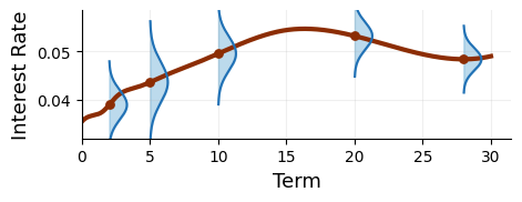
Term Structure Models

• In a rates exotics desk, we manage the joint movement of the entire curve

• The Challenge: We need one single model to parameterize the first 4 moments of distribution not just at one point, but the entire yield curve

def plot_forward_curve_with_vols(figsize=(6, 3.3)):
    import numpy as np
    import matplotlib.pyplot as plt
    from scipy.interpolate import CubicSpline

    fwd_knots = np.array([0.0, 0.5, 1.5, 2.5, 4.0, 6.0, 8.5, 15.0, 25.0, 30.0])
    fwd_vals  = np.array([0.0355, 0.0365, 0.0375, 0.04055, 0.04255, 0.0449, 0.04773, 0.0544, 0.0494, 0.0490])
    cs = CubicSpline(fwd_knots, fwd_vals, bc_type='not-a-knot')
    maturity = np.linspace(0, 30, 1201)
    forward_curve = cs(maturity)

    fig, ax = plt.subplots(figsize=figsize)
    ax.plot(maturity, forward_curve, color='#8c2d04', linewidth=3)

    pillars = np.array([2, 5, 10, 20, 28], dtype=float)
    pillar_forwards = cs(pillars)
    vols = np.array([0.0030, 0.0042, 0.0035, 0.0028, 0.0023])
    width_scale = 1.3

    for pillar, center, vol in zip(pillars, pillar_forwards, vols):
        move = np.linspace(-3 * vol, 3 * vol, 250)
        density = np.exp(-0.5 * (move / vol) ** 2)
        density /= density.max()
        x_right = pillar + width_scale * density
        ax.fill_betweenx(center + move, pillar, x_right, color='#6baed6', alpha=0.45)
        ax.plot(x_right, center + move, color='#2171b5', linewidth=1.5)
        ax.scatter([pillar], [center], color='#8c2d04', s=28, zorder=3)

    ax.set_xlim(0, 31.5)
    ax.set_ylim(0.032, 0.0585)
    ax.set_xlabel('Term', fontsize=13)
    ax.set_ylabel('Interest Rate', fontsize=13)
    ax.grid(alpha=0.2)
    for spine in ['top', 'right']:
        ax.spines[spine].set_visible(False)
    plt.show()

plot_forward_curve_with_vols()

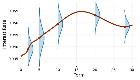
Heath–Jarrow–Morton (HJM) Framework

• Under the risk-neutral probability, once forward rate vol is determined, so is its drift

• \(f(t, T)\): Instantaneous forward rate for the reference period \([T, T+\epsilon]\) observed at \(t\)

• \(\sigma(t, T)\): Forward rate vol

• \({\color{lightgray}\Sigma(t, T) = \int_t^T\sigma(t, u)\,du: \text{zero coupon bond vol}}\)

  \[df(t, T) = {\color{lightgray} \sigma(t, T)\Sigma(t, T)\,dt} + \sigma(t, T)\,d\widetilde W(t), \qquad t<T\]

plot_forward_curve_with_vols(figsize=(5, 1.5))

• Think of a fixed \(T\), say 10Y

  \[df_{\text{10Y}}(t) = {\color{lightgray} \sigma_{\text{10Y}}(t)\Sigma_{\text{10Y}}(t)\,dt} + \sigma_{\text{10Y}}(t)\,d\widetilde W(t), \qquad t<\text{10Y}\]

HJM Is Not Optional

• To guarantee no arbitrage, any model for the instantaneous forward rate must have the drift term in the form as specified in the HJM framework

• But if you don’t model instantaneous forward rate, then HJM is irrelevant

  • An example is the LIBOR Market Model

• We only have to specify a \(\sigma(t, T)\) to obtain a concrete HJM model for pricing and hedging

• So how can we specify a \(\sigma(t, T)\)? Some properties:

  • Separable

  • Time stationary

  • Deterministic

Separable Vol

• A special class of HJM models where the volatility function is in the form

  \[\sigma(t, T) = g(t)h(T)\]

• Why does it matter?

• In an HJM model with separable vol, the forward rate is Markovian

• Markov Process: A random process’s future state only depends on its current state, not the past

  • Markovian example:

    \[E[X_{t+1}|\mathcal F_t] = E[X_{t+1}|X_t]\]

  • Non-Markovian example:

    \[E[X_{t+1}|\mathcal F_t] = E[X_{t+1}~|~X_t, X_{t-1}, X_{t-2}]\]

• Non-Markovian rates are path-dependent: dynamic hedging is infeasible, pricing is computationally explosive, and rate predictability opens the door to statistical arbitrage

Time Stationary Vol

• If the forward rate vol is a function of \(\tau = (T-t)\), we say it’s time stationary

• Why does it matter?

• Today’s 10Y forward rate vol is \(\sigma(0, 10)\)

• 1M from now, the same model gives the 10Y forward rate vol \(\sigma(\frac{1}{12}, 10 + \frac{1}{12})\)

• When \(\sigma(t, T)\) is time stationary, they are the same

• \(\tau = (T-t)\) is the term in a term structure model

• Time stationary vol means the vol stays constant for the same term when time \(t\) moves forward

• Without further information, time stationary vol is a good assumption

Gaussian HJM Model

• Assume that \(\sigma(t, T)\) is deterministic, giving normally distributed forward rates

  \[f(t, T) = {\color{lightgray} f(0, T) + \int_0^t\sigma(s, T)\Sigma(s, T)\,ds} + \int_0^t\sigma(s, T)\,d\widetilde W(s), \qquad t<T\]

• Examples:

  • Hull-White One Factor (HW1F)

    \[\sigma(t, T) = \sigma e^{-k(T-t)} = \sigma e^{-k\tau}\]

  • Ho-Lee: Constant forward rate vol, special case of HW1F with \(k\downarrow 0\)

    \[\sigma(t, T) = \sigma\]

• It can be shown that the only HJM model with separable, time stationary and deterministic vol is the Hull-White model (HWNF)

Curve Movement in the Ho-Lee Model

• Given \(\sigma(t, T) = \sigma\), at time \(t=0\), the forward rate evolves as \begin{align*} df(t, T) &= \sigma^2T\,dt + \sigma \,d\widetilde W(t) \\ &\approx {\color{darkcyan}\sigma^2\tau\Delta t} + {\color{red}\sigma (\widetilde W(\Delta t))} \end{align*}

• \(df(t, T)\) (as a function of \(T\)): Tomorrow’s forward curve movement

• \({\color{darkcyan}\sigma^2\tau\Delta t}\): An upward-sloping straight line, deterministic curve steepening

• \({\color{red}\sigma (\widetilde W(\Delta t))}\): Perfect parallel shift with random magnitude

• The Ho-Lee model implies that the curve is always steepening, albeit by a very small amount

HW1F

With \(\sigma(t, T) = \sigma e^{-\kappa \tau}\), the forward rate evolves as \begin{align*} df(t, T) &= {\color{lightgray}\sigma(t, T)\Sigma(t, T)\,dt} + \sigma(t, T)\,d\widetilde W(t)\\ &= {\color{lightgray}\left(y(t) - kx(t) + \frac{1-e^{-k\tau}}{k} (\sigma^2 - 2ky(t))\right)\,dt} + \sigma e^{-k\tau}\,d\widetilde W(t), \end{align*} where \({\color{lightgray}x(0) = y(0) = 0,}\) \begin{align*} {\color{lightgray} \begin{cases} dx(t) = (y(t) - \kappa x(t))dt + \sigma d\widetilde W(t)\\ dy(t) = (\sigma^2 - 2\kappa y(t)) dt \end{cases}. } \end{align*} The ODE of \({\color{lightgray}y(t)}\) can be solved explicitly to obtain

\[{\color{lightgray}y(t) = \frac{\sigma^2\left(1-e^{-2\kappa t}\right)}{2\kappa}, }\]

and the state variable \(x(t)\) is normally distributed.

Curve Movement in HW1F

At \(t=0\), tomorrow’s curve movement is \begin{align*} df(t, T) \approx \underbrace{\frac{\sigma^2(1-e^{-k\tau})}{k} \Delta t}_{\color{dodgerblue}(1)} + \underbrace{\sigma e^{-k\tau} \widetilde W(\Delta t)}_{\color{red}(2)} \end{align*}

• \({\color{red}(1)}\): Deterministic curve steepening

• \({\color{dodgerblue}(2)}\): Curve movement with random magnitude (\(\widetilde W(\Delta t) = \sqrt{\Delta t}Z\) below)

import numpy as np
import matplotlib.pyplot as plt
from ipywidgets import interact
import warnings
warnings.filterwarnings('ignore')

tau = np.linspace(0, 20, 1000)

@interact(sigma=(0.01, 0.5, 0.01), k=(0.01, 1, 0.01), Z=(-3, 3, 0.1))
def plot_curve_movement(sigma=0.2, k=0.4, Z=-1):
    s = sigma
    dt = 1/365

    drift = (s**2) * (1 - np.exp(-k * tau)) * dt / k
    diffusion = s * np.sqrt(dt) * np.exp(-k * tau) * Z
    total_movement = drift + diffusion

    fig, (ax1, ax2, ax3) = plt.subplots(1, 3, figsize=(15, 3.5))

    ax1.plot(tau, drift, linewidth=2, color='darkcyan')
    ax1.set_title('(1) Deterministic Steepening', color='darkcyan')
    ax1.set_xlim(0, 20)
    ax1.set_ylim(-0.1, 0.1)
    ax1.grid(True, alpha=0.3)
    ax1.set_xlabel(r'$\tau$')
    ax1.set_ylabel('Curve Movement')

    ax2.plot(tau, diffusion, linewidth=2, color='red')
    ax2.set_title('(2) Random Movement', color='red')
    ax2.set_xlim(0, 20)
    ax2.set_ylim(-0.1, 0.1)
    ax2.grid(True, alpha=0.3)
    ax2.set_xlabel(r'$\tau$')

    ax3.plot(tau, total_movement, linewidth=2, color='blue')
    ax3.set_title('Total Curve Movement', color='blue')
    ax3.set_xlim(0, 20)
    ax3.set_ylim(-0.1, 0.1)
    ax3.grid(True, alpha=0.3)
    ax3.set_xlabel(r'$\tau$')

    plt.tight_layout()
    plt.show()

HW2F and PCA

• At \(t=0\), tomorrow’s curve movement is \begin{align*} {\small df(t, T) \approx (\text{Deterministic Term}) + \underbrace{\left(\sigma_1 e^{-k_1\tau} + \rho\sigma_2e^{-k_2\tau}\right) \widetilde W_1(\Delta t)}_{\color{red}(1)} + \underbrace{\left(\sigma_2\sqrt{1-\rho^2} e^{-k_2\tau}\right) \widetilde W_2(\Delta t)}_{\color{dodgerblue}(2)}, } \end{align*} where \(\widetilde W_1(\Delta t) \perp\!\!\!\perp \widetilde W_2(\Delta t)\).

• \({\color{red}(1)}\): Curve movement contributed by PC1

• \({\color{dodgerblue}(2)}\): Curve movement contributed by PC2

Bond Reconstruction Formula

• In the Hull-White model, the zero coupon bond (ZCB) price \(P(t, T)\) is known in closed form in terms of the state variable(s)

  \[P(t, T) = P(t, T, x_t) {\color{lightgray} = \frac{P(0, T)}{P(0, t)} \exp\left(-G(t, T)x_t - \frac{1}{2}G^2(t, T)y_t\right), }\]

  where

  \[{\color{lightgray} G(t, T) = \frac{1-e^{k(T-t)}}{k}, \qquad y_t = \frac{\sigma^2(1-e^{2kt})}{2k}}\]

• Why is this useful?

• Many important quantities can be written in terms of ZCBs, including:

  • Forward rate \(L(t, T, T+\tau) = (P(t, T)/P(t, T+\tau) - 1)/\tau\)

  • Swap rate, as it’s a weighted average of forward rates. We denote this by \(S(t, x_t)\)

  • Annuity, as it’s a basket of ZCBs. We denote this by \(A(t, x_t)\)

Problem With HW

• Despite all the benefits of the Hull-White model, it doesn’t give us control over the 3rd and the 4th moments (IV skews and convexity)

• \(f(t, T)\) is normally distributed

• The swap rate \(S(t, x_t)\) is not, but there is no parameter for IV skew control

plot_forward_curve_with_vols()

From HW to Cheyette

\begin{align*} \begin{cases} dx_t = (y_t - \kappa x_t)dt + {\color{red}\sigma} d\widetilde W_t\\ dy_t = ({\color{red}\sigma}^2 - 2\kappa y_t) dt \end{cases} \end{align*}

• HW: Constant \(\sigma\)

• Cheyette: \(\sigma(t, x_t, y_t) = a_0 + a_1 x_t\)

• Similar to the displaced lognormal model, there is now a skew parameter \(a_1\)

• Since \(\sigma\) is random now, so is \(y_t\)

• Bond reconstruction formula still holds but with random \(y_t\):

  \[P(t, T) = P(t, T, x_t, y_t) {\color{lightgray} = \frac{P(0, T)}{P(0, t)} \exp\left(-G(t, T)x_t - \frac{1}{2}G^2(t, T)y_t\right), }\]

  where

  \[{\color{lightgray} G(t, T) = \frac{1-e^{k(T-t)}}{k}}\]

Cheyette Model With Stochastic Volatility

• Extension to SV gives us a vol of vol parameter \({\color{dodgerblue}\nu}\) to control the convexity of IV \begin{align*} \begin{cases} \color{lightgray}dx_t = (y_t - \kappa x_t)dt + {\color{black}\sqrt{\alpha_t}}\sigma(t, x_t, y_t) d\widetilde W_t\\ \color{lightgray}dy_t = ({\color{black}\alpha_t}\sigma^2(t, x_t, y_t) - 2\kappa y_t) dt\\ d\alpha_t = k(\theta - \alpha_t)\,dt + {\color{dodgerblue}\nu}\sqrt{\alpha_t}\,dZ_t \end{cases} \end{align*}

Appendix: Swaption Pricing in Cheyette

• Swap rate is now \(S(t, x_t, y_t)\), where \(S(\cdot, \cdot, \cdot)\) is a lengthy formula but in closed form

• To find swaption NPV approximation, we find swap rate dynamics approximation: \begin{align*} dS_t &= \frac{\partial S}{\partial x}(t, x_t, y_t)\,dx_t \\ &= \frac{\partial S}{\partial x}(t, x_t, y_t)\sigma(t, x_t, y_t)\,dW^A_t \end{align*}

• Replace \(y_t\) by \(\color{red}\bar y_t\), the deterministic function in HW:

  \[dS_t \approx \frac{\partial S}{\partial x}(t, x_t, {\color{red}\bar y_t})\sigma(t, x_t, {\color{red}\bar y_t})\,dW^A_t\]

• The right hand side is in terms of \(x_t\), not \(S_t\), which is undesired

\[dS_t \approx \frac{\partial S}{\partial x}(t, x_t, \bar y_t)\sigma(t, x_t, \bar y_t)\,dW^A_t\]

• Expand \(S(t, x, y)\) in \(x\) to the first order and find the inverse function as an approximation of \(x(t, S)\). Denote the inverse function by \(\xi(t, s)\). Next write

  \[dS_t \approx \underbrace{\frac{\partial S}{\partial x}(t, \xi(t, S_t), \bar y_t)\sigma(t, \xi(t, S_t), \bar y_t)}_{\text{RHS vol}}\,dW^A_t\]

• Find first order approximation \(\text{RHS vol} \approx a_0(t) + a_1(t) S_t\). Now we have a swap rate dynamics approximation which is displaced lognormal and can be used in pricing:

  \[dS_t \approx (a_0(t) + a_1(t) S_t)\,dW^A_t\]

# import numpy as np
# import matplotlib.pyplot as plt

# fig, ax = plt.subplots(figsize=(7, 5))

# # Use y = -T so the T-axis points downward on the page.
# t_max = 10
# T_max = 10

# t = np.linspace(0, t_max, 400)
# y_line = -t

# # Shade the region below the line t = T in the fourth quadrant.
# ax.fill_between(t, y_line, -T_max, color="#9ecae1", alpha=0.6)
# ax.plot(t, y_line, color="#08519c", linewidth=2.5)

# # Clean frame and draw custom axes.
# for spine in ax.spines.values():
#     spine.set_visible(False)

# ax.set_xlim(-0.5, t_max + 0.8)
# ax.set_ylim(-T_max - 0.8, 0.8)
# ax.set_xticks([])
# ax.set_yticks([])

# ax.annotate("", xy=(t_max + 0.5, 0), xytext=(0, 0),
#             arrowprops=dict(arrowstyle="->", linewidth=2, color="black"))
# ax.annotate("", xy=(0, -T_max - 0.5), xytext=(0, 0),
#             arrowprops=dict(arrowstyle="->", linewidth=2, color="black"))

# ax.text(t_max + 0.55, 0.15, r"$t$", fontsize=16)
# ax.text(-0.35, -T_max - 0.55, r"$T$", fontsize=16)
# ax.text(6.2, -5.3, r"$t = T$", color="#08519c", fontsize=14)
# ax.text(6.3, -8.8, "HJM domain", color="#08306b", fontsize=13)

# plt.show()