11. Interest Rate Swaps (IRS)

[2]:

from fixedincome2025 import table

Overview

Interest rate swap is by far the most liquid OTC product
In this chapter we introduce the standard SOFR swap and its pricing

Standard SOFR Swap

In a SOFR swap, two parties aggree on a term and a notional principal, say the term is 10y and the notional principal is 100 million
Party A agrees to pay party B a yearly interest determined by a fixed coupon rate, say $3.65\%$, on the the notional principal agreed upon at the end of every year for the following 10 years
In return, party B aggrees to pay party A a yearly interest determined by the 1y SOFR term rate:

\[\text{SOFR Term Rate} = \frac{1}{\tau}\left(\prod_j (1+\Delta t_j r_j) - 1\right),\]

with $\tau = 1$ for 1y. The payment is also made at the end of every year for the following 10 years
There is no principal payment on either side, that’s why it’s called the notional principal: No one has ever seen that 100 million
There is no initial payment on either side, but the fixed rates are quoted in the market for all terms up to 30 years

Standard SOFR Swap: Terminologies

Fixed Rate: The fixing coupon rate, $3.65\%$ in the previous examle
Floating Rate: Yearly SOFR term rate in the previous examle
Fixed Leg: All fixed coupon payments (cash flows)
Floating Leg: All floating coupon payments (cash flows)
Swap Legs: Fixed leg and floating leg
Payer Swap: If you are the party who pays fixed coupons, you say you have a payer swap
Receiver Swap: If you are the party who receives floating coupons, you have a receiver swap
Swap Rate: The fixed rate is called the swap rate of the term. For example $3.65\%$ would be the 10y swap rate in the previous example

Yield Curve’s 6 Representations With SOFR Extension

Given the backward looking nature of the SOFR term rate, a forward contract for the period $[T, T+\tau]$ can trade in the period $[T, T+\tau]$
- This wasn’t possible in the LIBOR world where the forward contract has the underlying forward rate fixed at $T$
Now we need to model $L(t, T, T+\tau)$ for $t\in [T, T+\tau]$

But recall that $L(t, T, T+\tau)$ is implied by \begin{align*} \frac{1}{1+\tau L(t, T, T+\tau)} = p(t, T, T+\tau) = \frac{P(t, T+\tau)}{P(t, T)} \end{align*}
Plugging in a $t$ that’s greater than $T$ breaks the definition:
- What’s the meaning of $P(t, T)$ when $t>T$?

[1]:

import matplotlib.pyplot as plt
import numpy as np

# Hexagon vertices (clockwise, starting from top left)
labels = [
    r"$P(t, T)$",
    r"$R(t, T)$",
    r"$r_t$",
    r"$f(t, T)$",
    r"$L(t, T, T+\tau)$",
    r"$P(t, T, T+\tau)$",
    ]

# Calculate hexagon coordinates
angles = np.linspace(np.pi/2 + np.pi/6, np.pi/2 + np.pi/6 + 2*np.pi, 7)  # 6 vertices + close the shape
radius = 1
x = radius * np.cos(angles)
y = radius * np.sin(angles)

fig, ax = plt.subplots(figsize=(6,6))
ax.plot(x, y, 'k-', lw=2)
ax.scatter(x[:-1], y[:-1], s=100, color='skyblue', zorder=5)

# Annotate each vertex with custom offset for the long label
for i, label in enumerate(labels):
    # Default offset
    dx = 0.18 * np.cos(angles[i])
    dy = 0.18 * np.sin(angles[i])
    # Increase offset for the long label 'L(t, T, T+tau)'
    if label == r"$L(t, T, T+\tau)$":
        dx *= 2
        dy *= 2
    elif label == "$R(t, T)$":
        dx *= 1.5
        dy *= 1.5
    ax.text(x[i]+dx, y[i]+dy, label, fontsize=14, ha='center', va='center')

ax.set_aspect('equal')
ax.axis('off')
# plt.title('Six Yield Curve Notations (Clockwise)', fontsize=16)
plt.show()

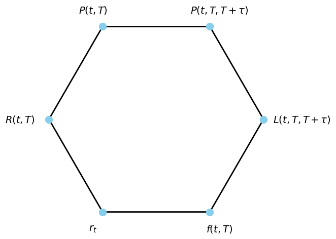
The 6 Representations of Yield Curve: Review

Money Market Account (MMA)

If you put $\$1$ into an MMA at time zero, the time-$t$ value of the account is \begin{align*} M_t = e^{\int_0^t r_s\,ds}, \end{align*} where $r_t$ is the short rate process
You can think of $r_t$ as the daily SOFR fixings
In an MMA you are simply lending out the cash nightly and keep rolling

Extended ZCB Price

For $t>T$, define \begin{align*} P(t, T) = \frac{M_t}{M_T} = e^{\int_T^t r_s\,ds} \end{align*}
This means, right after the maturity of the ZCB, you put the $\$1$ cash into an MMA

Extended Forward Rate

The forward term rate: \begin{align*} L(t, T, T+\tau) = \frac{1}{\tau} \left(\frac{P(t, T)}{P(t, T+\tau)} - 1\right) \end{align*}
When $t\in[T, T+\tau)$, the numerator $P(t, T) = e^{\int_T^t r_s\,ds}$ is known but the denominator $P(t, T+\tau)$ is still unknown so $L(t, T, T+\tau)$ is not fixed
- While the denominator $P(t, T+\tau)$ is unknown, it’s less and less volatile when $t$ gets closer and closer to $T+\tau$, consistent with our previous observation that the forward term rate is less and less volatile in the reference period
- This is different from the LIBOR world where $L(t, T, T+\tau)$ is fixed at $t=T$
At $t = T+\tau$, both numerator and denominator are known so $L(t, T, T+\tau)$ is fixed

Forward Rate Fixing

At $t \ge T+\tau$, the forward rate is fixed to be \begin{align*} L(t, T, T+\tau) &= \frac{1}{\tau} \left(\frac{P(t, T)}{P(t, T+\tau)} - 1\right)\\ &= \frac{1}{\tau} \left(\frac{M_t/M_T}{M_t/M_{T+\tau}} - 1\right)\\ &= \frac{1}{\tau} \left(e^{\int_T^{T+\tau} r_s\,ds} - 1\right)\\ &\approx \frac{1}{\tau} \left(e^{\sum_j r_{t_j}\Delta t_j} - 1\right)\\ &= \frac{1}{\tau} \left(\prod_j e^{r_{t_j}\Delta t_j} - 1\right)\\ &\approx \frac{1}{\tau} \left(\prod_j (1 + r_{t_j}\Delta t_j) - 1\right), \end{align*} which is the definition of the SOFR term rate

Extended Instantaneous Forward Rate

For $t>T$, the instantaneous forward rate is \begin{align*} f(t, T) &= -\frac{\partial}{\partial T} \log P(t, T)\\ &= -\frac{\partial}{\partial T} \int_T^t r_s\,ds = r_T, \end{align*} which is the daily SOFR fixing at $T$

Standard SOFR Swap Pricing

\[\]

\begin{align*} \text{Swap PV} &= \text{Floating Leg PV} + \text{Fixed Leg PV}\\ &= \sum_j(\text{PV of the $j$-th Floating Coupon Payment}) + \sum_j(\text{PV of the $j$-th Fixed Coupon Payment}) \end{align*}

PV of a Future Fixed Coupon Payment

Assuming the fixed rate is $K$, the time-$t$ PV of a future cash flow $\tau K$, received at time $T+\tau$, is

\[\tau P(t, T+\tau)K,\]

which is simply the discounted future cash flow

PV of a Future Floating Coupon Payment

PV of a future cash flow $\tau L(T+\tau, T, T+\tau)$, received at time $T+\tau$, can be derived from a no-arbitrage argument
If you buy $T$-ZCB and short sell $(T+\tau)$-ZCB at $t$:
- Your cost (net cash flow) at $t$ is $P(t, T+\tau) - P(t, T)$
- You are guaranteed to receive $\$1$ at $T$ and you are obligated to pay $\$1$ at $T+\tau$
- When you receive $\$1$ at $T$, lend it out in the repo market nightly, rolling the lending to a perid of $\tau$ years
- By $T+\tau$ you will have $1+\tau L(T+\tau, T, T+\tau)$
- But you are obligated to pay $\$1$ at $T+\tau$, so you are left with a net cash flow of $\tau L(T+\tau, T, T+\tau)$
In summary, $P(t, T+\tau) - P(t, T)$ is the cost at time $t$ to set up a risk-free portfolio in order to receive a future cash flow of $\tau L(T+\tau, T, T+\tau)$ at time $T+\tau$
That means the time-$t$ PV of a future cash flow $\tau L(T+\tau, T, T+\tau)$ received at time $T+\tau$ is $P(t, T) - P(t, T+\tau)$

PV of a Future Floating Coupon Payment (Cont.)

The time-$t$ PV of a future cash flow $\tau L(T+\tau, T, T+\tau)$ received at time $T+\tau$ is \begin{align*} P(t, T) - P(t, T+\tau) &= P(t, T+\tau)\left(\frac{P(t, T)}{P(t, T+\tau)} - 1\right)\\ &= P(t, T+\tau)\left(\frac{1}{P(t, T, T+\tau)}-1\right)\\ &= P(t, T+\tau)\left((1+\tau L(t, T, T+\tau))-1\right)\\ &= \tau P(t, T+\tau) L(t, T, T+\tau) \end{align*}
Compare this to the time-$t$ PV of a future fixed coupon payment: $\tau P(t, T+\tau)K$

Which one is more risky?

When rates move, since the bond price $P$ and forward rate $L$ move in different directions, the change in $\tau P(t, T+\tau) L(t, T, T+\tau)$ can be smaller than $\tau P(t, T+\tau)K$

This observation leads to a conclusion that’s maybe somewhat counterintuitive to beginners: Fixed legs can be more risky than floating legs

Dollar Durations

Recall that, since dollar duration times yield change approximately equals negative bond price change, an asset with large dollar duration is more risky
If you have a position with $\text{PV} =\tau K P(t, T+\tau)$, its dollar duration (term $\times$ bond price) is

\[D^{\$}_{\text{fixed}} = \tau K(T+\tau-t)P(t, T+\tau)\]
Dollar duration of a floating coupon payment is hard to compute from the formula

\[\tau P(t, T+\tau)L(t, T, T+\tau)\]
We look at the alternative form $P(t, T) - P(t, T+\tau)$. Its dollar duration is \begin{align*} D^{\$}_{\text{floating}} &= (T+\tau-t) P(t, T+\tau) - (T-t)P(t, T)\\ \end{align*}

\begin{align*} D^{\$}_{\text{floating}} &= (T+\tau-t) e^{-R(t, T+\tau)(T+\tau-t)} - (T-t)e^{-R(t, T)(T-t)}\\ &\approx (T+\tau-t) [1-R(t, T+\tau)(T+\tau-t)] - (T-t)[1-R(t, T)(T-t)]\\ &= \tau +R(t, T)(T-t)^2 - R(t, T+\tau)(T+\tau-t)^2 \end{align*}

Tenor Structure of a Swap

Define a tenor structure of a swap $T_0 < T_1 < T_2 < \cdots < T_N$
- At $T_0$, both parties enter into the swap with payment dates $T_1, T_2, \ldots, T_N$
Define $\tau_n = T_{n+1} - T_n$ for $n=0, 1, \ldots, N-1$
In a standard SOFR swap, $\tau_n$ is always 1y, and $T_n$ is the end of the $n$-th year

Swap Rate

The time-$T_0$ PV of an $N$-year-long (spot starting) payer swap with fixed rate $K$ is \begin{align*} \sum_{n=0}^{N-1}\left(\tau_n P(T_0, T_{n+1})L(T_0, T_n, T_{n+1}) - \tau_n P(T_0, T_{n+1})K\right) \end{align*}
As there is no initial payment, this PV is set to zero to find the swap rate $K^*$: \begin{align*} 0 &= \sum_{n=0}^{N-1}\left(\tau_n P(T_0, T_{n+1})L(t, T_n, T_{n+1}) - \tau_n P(T_0, T_{n+1})K^*\right)\\ &= \left[\sum_{n=0}^{N-1}\tau_n P(T_0, T_{n+1})L(T_0, T_n, T_{n+1})\right] - K^*\left[\sum_{n=0}^{N-1}\tau_n P(T_0, T_{n+1})\right], \end{align*} so \begin{align*} K^* = \frac{\sum_{n=0}^{N-1}\tau_n P(T_0, T_{n+1})L(T_0, T_n, T_{n+1})}{\sum_{n=0}^{N-1}\tau_n P(T_0, T_{n+1})} \end{align*}
This is the $N$-year swap rate quoted in the market

Swap Rate (Cont.)

\begin{align*} K^* = \frac{\sum_{n=0}^{N-1}\tau_n P(T_0, T_{n+1})L(T_0, T_n, T_{n+1})}{\sum_{n=0}^{N-1}\tau_n P(T_0, T_{n+1})} \end{align*}

A weighted average of the forward term rates, with the discount factors being the weights
- The closer the reference period $[T_n, T_{n+1}]$ is, the more heavily weighted the corresponding forward rate
The swap rate is uniquely determined by the current yield curve. Any quotes different from $K^*$ will lead to arbitrage

Swap Rate: Exercise I

If today’s SOFR yield curve is as below, what’s the 3Y swap rate?

[6]:

table('yc_10092025').T

[6]:

	1m	1.5m	2m	3m	4m	6m	1y	2y	3y	5y	7y	10y	20y	30y
Yield	4.2%	4.17%	4.11%	4.03%	3.95%	3.83%	3.66%	3.6%	3.59%	3.74%	3.92%	4.14%	4.7%	4.72%

Swap Curve

The swap rate depends on the tenor structure (depends on $N$)
For each term $N=1, 2, 3, \ldots, 30,$ we can compute a different swap rate $K^*$, which form the swap curve

Forward Swap Rate

In general, the time-$t$ PV of an $N$-year-long forward starting payer swap with fixed rate $K$ is \begin{align*} \sum_{n=0}^{N-1}\left(\tau_n P(t, T_{n+1})L(t, T_n, T_{n+1}) - \tau_n P(t, T_{n+1})K\right) \end{align*}
Following the same derivation as we’ve done previously, we obtain the formula for a forward swap rate, which we denote by $S(t)$ hereafter \begin{align*} S(t) = \frac{\sum_{n=0}^{N-1}\tau_n P(t, T_{n+1})L(t, T_n, T_{n+1})}{\sum_{n=0}^{N-1}\tau_n P(t, T_{n+1})} \end{align*}
The spot swap rate is $S(T_0)$
$S(t)$ is a weighted average of forward rates, both the weights and the forward rates are random, and they are related in a complex way
The forward swap rate is uniquely determined by the current yield curve, same as the spot swap rate, and the forward term rate $L(t, T, T+\tau)$

Annuity

Define the annuity process as the denominator of $S(t)$: \begin{align*} A(t) = \sum_{n=0}^{N-1}\tau_n P(t, T_{n+1}) \end{align*}
This is the time-$t$ PV of a financial product that promises to pay $\$1$ at the end of every year (at times $T_1, T_2, \ldots, T_N$), hence the name

Forward Starting Swap PV Clean Form

The time-$t$ PV of an $N$-year-long forward starting payer swap with fixed rate $K$ can be written as \begin{align*} &\sum_{n=0}^{N-1}\left(\tau_n P(t, T_{n+1})L(t, T_n, T_{n+1}) - \tau_n P(t, T_{n+1})K\right)\\ =& \left[\sum_{n=0}^{N-1}\tau_n P(t, T_{n+1})L(t, T_n, T_{n+1})\right] - K\left[\sum_{n=0}^{N-1}\tau_n P(t, T_{n+1})\right] \\ =& \left(\sum_{n=0}^{N-1}\tau_n P(t, T_{n+1})\right)\left(\frac{\sum_{n=0}^{N-1}\tau_n P(t, T_{n+1})L(t, T_n, T_{n+1})}{\sum_{n=0}^{N-1}\tau_n P(t, T_{n+1})} - K\right) \\\\ =& A(t)(S(t) - K) \end{align*}

Swap PV01

Previously we have mentioned PV01, the present value of 1bp, which is the PV change with 1 bp rates change
To compute PV01 of a swap first write down its PV:
- The time-$t$ PV of an forward starting payer swap with fixed rate $K$ is $A(t)(S(t) - K)$
- Plug in $t=T_0$ to obtain the spot starting swap PV $A(T_0)(S(T_0) - K)$
- But market will quote $K=S(T_0)$ so that no cash flows happen initially
- Initially, the PV is $A(T_0)(S(T_0) - K) = 0$
Imagine you have bought a swap at $T_0$ with zero PV initially. After a tiny $\Delta t$, if the swap rate is up 1bp, the PV becomes

\[A(T_0 + \Delta t)\underbrace{(S(T_0 + \Delta t) - K)}_{\approx 1 \text{ bp}} \approx A(T_0)\times 0.0001\]
Thus PV01 of a swap is approximately its corresponding annuity $A(T_0)$ times 1 bp

Swap PV01: A Closer Look

You bought a swap with zero PV initially, and after a tiny $\Delta t$, the swap rate is up 1bp
But swap rate is

\[S(t) = \frac{\sum_{n=0}^{N-1}\tau_n P(t, T_{n+1})L(t, T_n, T_{n+1})}{\sum_{n=0}^{N-1}\tau_n P(t, T_{n+1})}\]
If all forward rates $L(t, T_n, T_{n+1})$ are up 1 bp, the swap rate will be up approximately 1 bp
- “Approximately” because when forward rates change, ZCBs $P(t, T_n)$ also change
- So we are saying a parallel forward curve shift of 1 bp will lead to 1 bp shift in swap rate
- Previously we define PV01 to be PV change corresponding to parallel zero curve shift of 1 bp, not exactly the same
- There is not a rigorous definition of PV01, as in what rates are up by 1bp? Because there is no need. For one thing, the curve never really moves parallelly
Despite all that, $A(T_0)\times 0.0001$ is usually a good approximation of swap PV01 in practice

Swap Rate Alternative Formula

\[\]

\[S(t) = \frac{\sum_{n=0}^{N-1}\tau_n P(t, T_{n+1})L(t, T_n, T_{n+1})}{A(t)}, \qquad A(t) = \sum_{n=0}^{N-1}\tau_n P(t, T_{n+1})\]

In the formula we can replace $L(t, T_n, T_{n+1})$ by \begin{align*} L(t, T_n, T_{n+1}) = \frac{1}{\tau_n} \left(\frac{P(t, T_n)}{P(t, T_{n+1})} - 1\right) \end{align*} and write \begin{align*} S(t) &= \frac{\sum_{n=0}^{N-1}\tau_n P(t, T_{n+1})\left[\frac{1}{\tau_n} \left(\frac{P(t, T_n)}{P(t, T_{n+1})} - 1\right)\right]}{A(t)}\\ &= \frac{\sum_{n=0}^{N-1}\left(P(t, T_0) - P(t, T_{n+1})\right)}{A(t)}\\ &= \frac{P(t, T_0) - P(t, T_{N})}{A(t)} \end{align*}

Swap Rate Alternative Formula (Cont.)

The numerator simplifies to

\[\sum_{n=0}^{N-1}\tau_n P(t, T_{n+1})L(t, T_n, T_{n+1}) = P(t, T_0) - P(t, T_{N})\]
Previously in computing PV of a future floating coupon payment, we have seen a special case of this with $N=1$

Swap Rate Alternative Formula (Cont..)

We have \begin{align*} A(t) &= \sum_{n=0}^{N-1}\tau_n P(t, T_{n+1})\\ S(t) &= \frac{\sum_{n=0}^{N-1}\tau_n P(t, T_{n+1})L(t, T_n, T_{n+1})}{A(t)}\\ &= \frac{P(t, T_0) - P(t, T_N)}{A(t)} \end{align*}
In particular, we have the spot swap rate \begin{align*} S(T_0) = \frac{1 - P(T_0, T_{N})}{A(T_0)} \end{align*}

Swap Rate: Exercise II

Given a SOFR yield curve as below, what’s the 3Y swap rate?

[5]:

table('yc_10022025').T

[5]:

	1 Mo	1.5 Mo	2 Mo	3 Mo	4 Mo	6 Mo	1 Yr	2 Yr	3 Yr	5 Yr	7 Yr	10 Yr	20 Yr	30 Yr
10/2/2025	4.23%	4.18%	4.11%	4.02%	3.96%	3.81%	3.62%	3.55%	3.56%	3.67%	3.86%	4.10%	4.66%	4.69%

No Arbitrage Argument

Below is a no arbitrage argument of the identity

\[\sum_{n=0}^{N-1}\tau_n P(T_0, T_{n+1})L(T_0, T_n, T_{n+1}) = 1 - P(t, T_{N})\]
If you short sell an $N$-year ZCB with notional $\$1$, and you lend out $\$1$ today, your net cash flow today is the negative right-hand side $P(t, T_{N}) - 1$

No Arbitrage Argument (Cont.)

\[\]

\[\sum_{n=0}^{N-1}\tau_n P(T_0, T_{n+1})L(T_0, T_n, T_{n+1}) = 1 - P(t, T_{N})\]

If you lend out $\$1$ at floating rate for a year, at the end of the first year you receive $1+\tau_0 L(T_1, T_0, T_1)$. You keep the interest $\tau_0 L(T_1, T_0, T_1)$ and lend out the principal $\$1$ again at floating rate for the second year
At the end of the second year you receive $1+\tau_1 L(T_2, T_1, T_2)$. You keep the interest $\tau_1 L(T_2, T_1, T_2)$ and lend out the principal $\$1$ again at floating rate for the third year
If you keep doing this for $N$ years, you get interest cash flows $\tau_n L(T_{n+1}, T_n, T_{n+1})$ at the end of the $(n+1)$-th year, for all $n=0, 1, \ldots, N-1$
At the end of the $N$-th year, you keep the interest $\tau_{N-1} L(T_{N}, T_{N-1}, T_{N})$ and use the $\$1$ to clear the ZCB you sold at the beginning
But we have established that, the time-$T_0$ PV of $\tau_n L(T_{n+1}, T_n, T_{n+1})$ is $\tau_n P(T_0, T_{n+1})L(T_0, T_n, T_{n+1})$
Thus we must have PVs of all interest cash flows sum up (left-hand side) to be the initial cost setting up this strategy (right-hand side)

Synthetic Fixed-Rate Bond

Swaps provide a way to lock in the fixed rate for a series of periodical interest payment, like holding a fixed coupon bond
If you have $\$1$ notional, this is how you can lock in the 5Y swap rate quoted in the market today, for the following 5 years:
- Run the “keep lending out $\$1$ to earn the interest at the end of every year” strategy to get a series of floating interest payments
- Enter into a 5Y receiver swap to trade floating interest for fixed coupon interest payments

Swap Spread

But you could have just bought the 5Y Treasuries. What’s the difference?

\[\text{5Y Swap Spread} = \text{5Y Swap Rate} - \text{5Y Treasury Yield}\]
Swap spreads at different terms form a spread curve, mostly positive. Does that give you an arbitrage opportunity?

No! As explained in the early chapters, Treasury yields are artificially low given tax benefit and regulatory requirements
If you short sell a 5Y treasury note to finance a 5Y synthetic fixed-rate bond in the swap market, given the positive swap spread, you might think you can earn interests at a higher 5Y swap rate while paying treasury coupons at a lower rate, but because of income tax, you end up making very little, or lose money

Constant Maturity Swap (CMS)

Standard SOFR swaps are so liquid the swap rates itself is an index upon which people trade derivatives (CMS swaps, CMS options, etc.)
Think of a fixed term, say 10y. We have $N=10$ and \begin{align*} A(T_0) = \sum_{n=0}^{N-1}\tau_n P(T_0, T_{n+1}), \qquad S(T_0) = \frac{1 - P(T_0, T_{N})}{A(T_0)} \end{align*}
Think of all $T_n$ some calendar dates, say $T_0$ is 11/19/2025, $T_1$ is 11/19/2026, etc.
At EOD 11/19/2025, when we have a close curve, all ZCBs, and hence $S(T_0)$ are known and fixed
The next day, we use the same formula but with $T_0$ being 11/20/2025, $T_1$ being 11/20/2026, etc.
At EOD 11/20/2025, when we have a close curve, $S(T_0)$ is known and fixed to be a different number as 11/19’s 10y swap rate close quote
Thus we obtain a 10y swap rate every day, that’s known as the 10y CMS rate
Derivatives on 2y, 5y, 10y, and 30y CMS rates are more liquidly trading