1. Yield Curve and Its 6 Representations

Interest Rate

Interest is the cost of borrowing paid by the borrower to the lender in order to compensate the inconvenience when the lender doesn’t have the cash at hand
Interest is not just about default risk; Even if a borrower has absolutely no chance to default, there will still be a cost for him/her to borrow
Interest rate is interest divided by notional, usually annualized

Term Structure

Borrowing for short term (say 1Y) and long term (say 10Y) usually have different costs

Data from treasury.gov

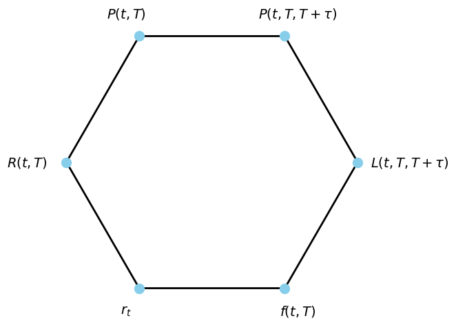
The 6 Representations of Yield Curve

[3]:

import matplotlib.pyplot as plt
import numpy as np

# Hexagon vertices (clockwise, starting from top left)
labels = [
    r"$P(t, T)$",
    r"$R(t, T)$",
    r"$r_t$",
    r"$f(t, T)$",
    r"$L(t, T, T+\tau)$",
    r"$P(t, T, T+\tau)$",
    ]

# Calculate hexagon coordinates
angles = np.linspace(np.pi/2 + np.pi/6, np.pi/2 + np.pi/6 + 2*np.pi, 7)  # 6 vertices + close the shape
radius = 1
x = radius * np.cos(angles)
y = radius * np.sin(angles)

fig, ax = plt.subplots(figsize=(6,6))
ax.plot(x, y, 'k-', lw=2)
ax.scatter(x[:-1], y[:-1], s=100, color='skyblue', zorder=5)

# Annotate each vertex with custom offset for the long label
for i, label in enumerate(labels):
    # Default offset
    dx = 0.18 * np.cos(angles[i])
    dy = 0.18 * np.sin(angles[i])
    # Increase offset for the long label 'L(t, T, T+tau)'
    if label == r"$L(t, T, T+\tau)$":
        dx *= 2
        dy *= 2
    elif label == "$R(t, T)$":
        dx *= 1.5
        dy *= 1.5
    ax.text(x[i]+dx, y[i]+dy, label, fontsize=14, ha='center', va='center')

ax.set_aspect('equal')
ax.axis('off')
# plt.title('Six Yield Curve Notations (Clockwise)', fontsize=16)
plt.show()

The 6 Representations of Yield Curve (Cont.)

Zero Rate and Zero-Coupon Bond Price

Zero rate $R(t, T)$ is defined to be the solution of

\[P(t, T) = e^{-R(t, T)(T-t)}\]
In usual market conditions we have $P(t, T) < 1$, which is equivalent to $R(t, T) > 0$

In the US Treasury example, we have $t =$ 2025/9/5
For $T-t =$ 10Y, we have $R(t, T) = 4.1\%$
Zero-coupon bond price is

\[P(t, T) = e^{-R(t, T)(T-t)} = e^{-0.041\times 10} \approx 0.6637\]

Zero-Coupon Bond Price

Exercise: What is 5Y ZCB price?

Zero-Coupon Bond Price as a Discount Factor

$P(t, T)$ is the time-$t$ price of a ZCB that promises to pay $\$1$ at $T$
Buying such a ZCB at $t$, you have
- Cash outflow $P(t, T)$ at $t$
- Cash inflow $\$1$ at $T$

You can scale this trade by $\$M$ and get
- Cash outflow $MP(t, T)$ at $t$
- Cash inflow $\$M$ at $T$

Cash flow at $t$ is cash flow at $T$ discounted (recall that $P(t, T) < 1$) \begin{align*} &(\text{Cash flow at }t) = (\text{Cash flow at }T)\times P(t, T)\\ &(\text{Cash flow at }T) = (\text{Cash flow at }t)/P(t, T)\\ \end{align*}

This will be useful in the no arbitrage argument deriving forward bond price
This is why $P(t, T)$ is sometimes referred to as the discount factor
- Not to be confused with the discounting process $D_t = e^{-\int_0^t r_s\,ds}$

Forward Rate and Forward Bond Price

If, at time $t$, you can foresee you will want to borrow in a future period of time, you can lock in the rate today
The rate you see today, computed from today’s yield curve, is the forward rate $L(t, T, T+\tau)$

Forward Bond Price

Say you know you will want to borrow 2Y from now, and return $\$1$ at 3Y from now, so the future period $[T, T+\tau]$ is [2Y, 3Y]

This is how you can lock in the rate today:
- Short sell 3Y ZCB that promises to pay $1$ and get cash $0.9009$ (equivalent to borrowing $0.9009$ and returning $1$ in 3Y)
- Use the cash $0.9009$ to buy 2Y ZCB that promises to pay $0.9009/0.9322 = 0.9664$ (equivalent to lending $0.9009$ out for 2Y and expecting $0.9664$ in return)
You end up with cash inflow $\$0.9664$ at 2Y and cash outflow $\$1$ at 3Y
This is called short selling a forward bond for the future period [2Y, 3Y] at $0.9664$, which is the forward bond price $P(t, T, T+\tau)$

Forward Bond Price: Exercise

What is the forward bond price for the future period [5Y, 7Y]

$0.7664/0.8357 = 0.9171$

Notations

$t =$ today
$T =$ 2Y
$T+\tau =$ 3Y
$P(t, T) = 0.9322$
$P(t, T+\tau) = 0.9009$
Forward bond price

\[P(t, T, T+\tau) = \frac{P(t, T+\tau)}{P(t, T)} = 0.9664\]

How To Arbitrage if the Quote Is Off

If, on 9/5/2025, a banker undervalued the [2Y, 3Y] forward bond and quoted you $0.95$, then you should
1. Short sell one unit of 3Y ZCB and get cash $0.9009$ (equivalent to borrowing $0.9009$ today and returning $1$ in 3Y)
2. Use the cash $0.9009$ to buy 2Y ZCB paying $0.9009/0.9322 = 0.9664$ (equivalent to lending $0.9009$ out for 2Y and expecting $0.9664$ in return)
3. Buy the forward bond from the banker at $0.95$
You end up with
- Cash inflow $\$0.9664$ at 2Y and cash outflow $\$1$ at 3Y from steps 1 and 2
- Cash outflow $\$0.95$ at 2Y and cash inflow $\$1$ at 3Y from step 3
- Sum up to a free cash inflow of $\$0.0164$ at 2Y

Or equivalently, today’s profit

\[0.0164\times 0.9322 = \$0.01529\]

No Arbitrage Principle

In reality you will never see an arbitrage opportunity in the market

How To Arbitrage if the Quote Is Off: Exercise

Exercise: If a banker overvalued the [2Y, 3Y] forward bond and quoted you $0.97$, what should you do? And how much profit can you make today?

Buy one unit of 3Y ZCB, paying $0.9009$ (equivalent to lending $0.9009$ and have $1$ returned in 3Y)
Short sell 2Y ZCB paying $0.9009/0.9322 = 0.9664$ at the end and get cash $0.9009$ (equivalent to borrowing $0.9009$ today and returning $0.9664$ in 2Y)
Short sell the forward bond to the banker at $0.97$

You end up with
- Cash outflow $\$0.9664$ at 2Y and cash inflow $\$1$ at 3Y from steps 1 and 2
- Cash inflow $\$0.97$ at 2Y and cash outflow $\$1$ at 3Y from step 3
- Sum up to a free cash inflow of $\$0.0036$ at 2Y, or equivalently $0.0036\times 0.9322 = \$0.0034$ today

Forward Rate

You’d naturally wonder what’s the rate of the [2Y, 3Y] forward bond
The answer is the forward rate $L(t, T, T+\tau)$, defined as the solution of

\[P(t, T, T+\tau) = \frac{1}{1+\tau L(t, T, T+\tau)}\]
Equivalently,

\[L(t, T, T+\tau) = \frac{1}{\tau}\left(\frac{1}{P(t, T, T+\tau)} - 1\right) = \frac{1}{0.9664} - 1 = 3.477\%\]

Forward Rate: Exercise

What’s the forward rate for the future period [5Y, 7Y]?

\[L(t, T, T+\tau) = \frac{1}{\tau}\left(\frac{1}{P(t, T, T+\tau)} - 1\right) = \frac{1}{2}\left(\frac{1}{0.9171} - 1\right) = 4.52\%\]

Application of Forward Rate

One application of the forward rate is to compare the cost of borrowing
You know the [2Y, 3Y] forward bond has fair price $0.9664$ and the [5Y, 7Y] forward bond has fair price $0.9171$, but you can’t compare the prices as one bond is 1Y long and the other is 2Y. This is not apple to apple comparison
After omputing the forward rates, you know the [2Y, 3Y] forward bond is cheaper

Alternative to Forward Bond

Today you foresee you will want to borrow for the future period [2Y, 3Y]
You can either
- Short sell a forward bond
- Do nothing and wait 2Y, and borrow then (short selling a 1Y bond then)
Which one is better?

Don’t know, as the interest rate in 2Y is not predictable

More Alternatives

Do nothing today, and short sell a forward bond for the future period [2Y-1D, 3Y-1D] tomorrow
Do nothing today and tomorrow, and short sell a forward bond for the future period [2Y-2D, 3Y-2D] the day after
Do nothing today, tomorrow and the day after, and short sell a forward bond for the future period [2Y-3D, 3Y-3D] 3 days from now
…

Forward Rate Agreements

When a future period of time $[T, T+\tau]$ is specified, so far we have learned:
- The forward bond price is uniquely determined from today’s zero curve assuming no arbitrage
- A forward bond price has a corresponding forward rate; Given one it’s easy to compute the other

Given $[T, T+\tau]$, banks do not quote forward bond price, only the forward rate
This is called a forward rate agreement (FRA), an over-the-counter (OTC) product
Call a banker and say “I want to borrow $\$M$ at $T$ and return at $T+\tau$, what’s the interest rate you will charge?”
Say you call 10 different banks, and get 10 quotes. They should all be very close, or otherwise there is an arbitrage

FRA is not only a traded product in the real world, but also a building block for many more complicated rates products, conceptually important for interest rate derivatives pricing

Instantaneous Forward Rate

Taking $\tau\downarrow 0$, the forward rate $L(t, T, T+\tau)$ becomes the instantaneous forward rate $f(t, T)$
Forward rate $L(t, T, T+\tau)$ is the rate you see at $t$ for the future period $[T, T+\tau]$
Instantaneous forward rate $f(t, T)$ is the rate you see at $t$ for the future instant $[T, T+\epsilon]$
No one ever quotes instantaneous forward rates, but it is the fundamental of many interest rate models

Instantaneous Forward Rate From ZCB Price

\[\]

\begin{align*} f(t, T) &= \lim_{\tau \downarrow 0} L(t, T, T+\tau) \\ &= \lim_{\tau \downarrow 0} \frac{1}{\tau}\left(\frac{1}{P(t, T, T+\tau)} - 1\right) \\ &= \lim_{\tau \downarrow 0} \frac{1}{\tau}\left(\frac{P(t, T)}{P(t, T+\tau)} - 1\right) \\ &= \lim_{\tau \downarrow 0} \frac{1}{\tau}\left(\frac{P(t, T) - P(t, T+\tau)}{P(t, T+\tau)}\right) \\ &= \lim_{\tau \downarrow 0} \left(-\frac{1}{P(t, T+\tau)}\right)\left(\frac{P(t, T+\tau) - P(t, T)}{\tau}\right) \\ &= -\frac{1}{P(t, T)}\frac{\partial }{\partial T} P(t, T)\\ &= -\frac{\partial }{\partial T} \log P(t, T)\\ \end{align*}

Instantaneous Forward Rate From Zero Rate

\[\]

Note that \begin{align*} f(t, T) &= -\frac{\partial }{\partial T} \log P(t, T) = \frac{\partial }{\partial T} [(T-t)R(t, T)]. \end{align*} Plug in $t=0$ to obtain \begin{align*} f(0, T) = \frac{d }{d T} [TR(0, T)]. \end{align*} The quantity $TR(0, T)$ is called the time weighted zero rate. This identity means today’s instantaneous forward curve is today’s time weighted zero curve taking derivative. This is a useful fact in curve construction.

ZCB Price From Instantaneous Forward Rate

\[\]

Recall that \begin{align*} f(t, T) = -\frac{\partial }{\partial T} \log P(t, T). \end{align*} So \begin{align*} \log P(t, T) = -\int_c^T f(t, u)\,du \end{align*} for some constant $c$, but when $T=t$ we must have \begin{align*} 0 = \log P(t, t) = -\int_c^t f(t, u)\,du. \end{align*} Thus we have $c=t$ and hence \begin{align*} P(t, T) = e^{-\int_t^T f(t, u)\,du}. \end{align*}

Zero Rate From Instantaneous Forward Rate

\[\]

Recall that \begin{align*} e^{-(T-t)R(t, T)} = P(t, T) = e^{-\int_t^T f(t, u)\,du}. \end{align*} Thus \begin{align*} R(t, T) = \frac{1}{T-t}\int_t^T f(t, u)\,du. \end{align*} We could have obtained the same formula by integrating \begin{align*} f(t, T) = \frac{\partial }{\partial T} [(T-t)R(t, T)] \end{align*} which we just derived.

Forward Bond Price From Instantaneous Forward Rate

\[\]

Recall that \begin{align*} P(t, T) = e^{-\int_t^T f(t, u)\,du}. \end{align*} Thus \begin{align*} P(t, T, T+\tau) = \frac{P(t, T+\tau)}{P(t, T)} = e^{-\int_T^{T+\tau} f(t, u)\,du}. \end{align*}

Forward Term Rate From Instantaneous Forward Rate

\[\]

Since \begin{align*} P(t, T, T+\tau) = e^{-\int_T^{T+\tau} f(t, u)\,du}, \end{align*} we have \begin{align*} L(t, T, T+\tau) &= \frac{1}{\tau}\left(\frac{1}{P(t, T, T+\tau)} - 1\right) \\ &= \frac{1}{\tau}\left(e^{\int_T^{T+\tau} f(t, u)\,du} - 1\right). \end{align*}

ZCB Price and Zero Rate

\[\]

By definition we have

\[P(t, T) = e^{-R(t, T)(T-t)}.\]

We can isolate $R(t, T)$ to get

\[R(t, T) = -\frac{1}{T-t}\log P(t, T).\]

Forward Bond Price and Forward Rate

\[\]

By definition we have

\[P(t, T, T+\tau) = \frac{1}{1+\tau L(t, T, T+\tau)}.\]

We can isolate $L(t, T, T+\tau)$ to get

\[L(t, T, T+\tau) = \frac{1}{\tau}\left(\frac{1}{P(t, T, T+\tau)} - 1\right).\]

Appendix – Simple and Continuous Compounding

Simple Compounding

Assuming flat yield curve with annualized interest rate $r=2\%$
Certificate of Deposit (CD) with 1Y maturity: Save $1$ dollar (principal) in a bank for one year

\[1+r = 1.02\]
CD with 6M maturity: What if you put the money in the bank only for half a year?

\[1+\frac{r}{2} = 1.01\]
Rolling 6M CD: What if you roll the principal and earned interest from the current 6M CD into a new one?

\[\left(1+\frac{r}{2}\right)^2 = 1.0201 > 1+r\]

Simple Compounding (Cont.)

What if you put the money in the bank only for 1/3 year?
- CD with 4M maturity
  
  \[1+\frac{r}{3} \approx 1.00667\]
Rolling 4M CD

\[\left(1+\frac{r}{3}\right)^3 \approx 1.02013363\]
This is greater than rolling 6M CD

\[\left(1+\frac{r}{2}\right)^2 = 1.0201\]

[4]:

from pandas import DataFrame

r = 0.02

columns=['Rolling Frequency', 'Terminal Account Value']

DataFrame([(n, (1 + r/n)**n) for n in range(1, 11)],
          columns=columns).set_index('Rolling Frequency')

[4]:

	Terminal Account Value
Rolling Frequency
1	1.020000
2	1.020100
3	1.020134
4	1.020151
5	1.020161
6	1.020167
7	1.020172
8	1.020176
9	1.020179
10	1.020181

From Simple to Continuous

The more frequently you roll the CDs in a year, the higher the terminal account value will be
When rolling frequency goes to infinity, will the terminal account value goes to infinity?

No

\[\lim_{n\rightarrow\infty}\left(1+\frac{r}{n}\right)^n = e^r\]

Continuous Compounding

Repeatedly rolling 6M CDs for $T=5$ years, the terminal value is

\[\left(1+\frac{r}{2}\right)^{2\times 5}\]
Take the rolling frequency to infinity:

\[\lim_{n\rightarrow\infty}\left(1+\frac{r}{n}\right)^{nT} = e^{rT}\]
This is why zero rate $R(t, T)$ is defined as the solution of $P(t, T) = e^{-R(t, T)(T-t)}$