12. SOFR Yield Curve Construction
[26]:
from fixedincome2025 import table
Overview
The SOFR yield curve is by far the most important curve if you work in a bank’s rates business
Most OTC products, e.g. swaps, use SOFR as the index rate
In this chapter, we study the SOFR yield curve construction
As we will see now, it is very different from Treasury yield curve construction
Curve Instruments
Unlike Treasury yield curve which is constructed from the Treasuries, there is no SOFR bonds
The SOFR yield curve is constructed from
Daily SOFR fixing for the day
3M SOFR futures
Standard SOFR swaps
3M SOFR futures and standard SOFR swaps are the most liquid rates instruments linked to the SOFR index
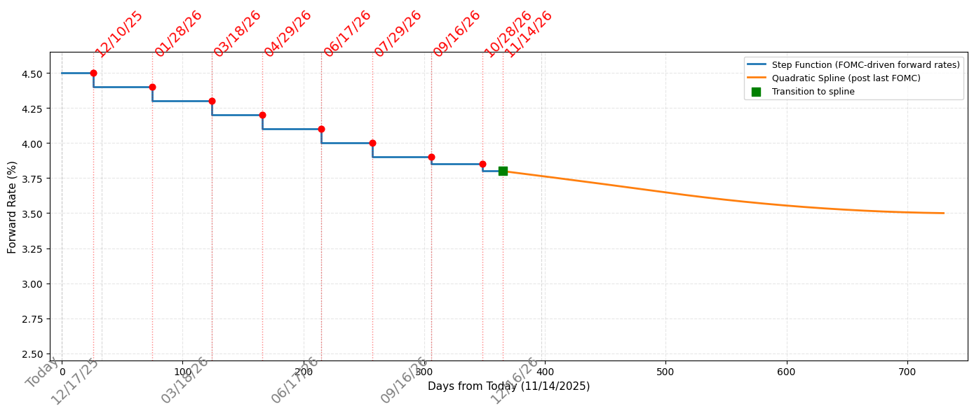
Curve Interpolation
Numerical settings same as explained in Curve Interpolation
Linear interpolation on the time weighted zero rate \(TR(0, T)\) at the short end
Cubic spline interpolated \(TR(0, T)\) for the rest of the curve
Which implies piecewise constant instantaneous forward rate \(f(0, T)\) at the short end and quadratic spline \(f(0, T)\) for the rest
Recall that
\[f(0, T) = \frac{d}{dT}[TR(0, T)]\]
Market Data
[69]:
table('curve_instruments')
[69]:
| Instrument | Quote | Convexity (bps) | |
|---|---|---|---|
| Deposit | 3.9700 | ||
| Futures Sep 25 | 95.9010 | 0 | |
| Futures Dec 25 | 96.1825 | 0.015563 | |
| Futures Mar 26 | 96.3925 | 0.091519 | |
| Futures Jun 26 | 96.6275 | 0.207215 | |
| Futures Sep 26 | 96.7875 | 0.362651 | |
| Swap 1y | 3.6151 | ||
| Swap 2y | 3.3980 | ||
| Swap 3y | 3.3624 | ||
| Swap 5y | 3.4232 | ||
| Swap 7y | 3.5379 | ||
| Swap 10y | 3.7120 | ||
| Swap 20y | 4.0420 | ||
| Swap 30y | 4.0199 |
Forward Rates
For each futures contract, the corresponding convexity adjustment is quoted, and we first compute forward rates by
\[\text{Forward Rate} = \text{Futures Rate} - \text{Convexity Adjustment}\]
[59]:
table('forward_rates')
[59]:
| Instrument | Quote (%) | |
|---|---|---|
| Futures Sep 25 | 4.100 | |
| Futures Dec 25 | 3.818 | |
| Futures Mar 26 | 3.608 | |
| Futures Jun 26 | ? | |
| Futures Sep 26 | ? |
Next we list the dates and compute year fractions
[51]:
table('key_dates')
[51]:
| Integer Year Fraction | IMM Dates | FOMC Meeting Dates | From Prev Key Date (Days) | From Today (Days) | Year Fraction | |
|---|---|---|---|---|---|---|
| 9/17/2025 | 9/17/2025 | 0 | -58 | -0.1589 | ||
| 10/29/2025 | 42 | -16 | -0.0438 | |||
| 11/14/2025 | 16 | 0 | 0.0000 | |||
| 12/10/2025 | 26 | 26 | 0.0712 | |||
| 12/17/2025 | 7 | 33 | 0.0904 | |||
| 1/28/2026 | 42 | 75 | 0.2055 | |||
| 3/18/2026 | 3/18/2026 | 49 | 124 | 0.3397 | ||
| 4/29/2026 | 42 | 166 | 0.4548 | |||
| 6/17/2026 | 6/17/2026 | 49 | 215 | 0.5890 | ||
| 7/29/2026 | 42 | 257 | 0.7041 | |||
| 9/16/2026 | 9/16/2026 | 49 | 306 | 0.8384 | ||
| 10/28/2026 | 42 | 348 | 0.9534 | |||
| 11/14/2026 | 17 | 365 | 1.0000 | |||
| 12/9/2026 | 25 | 390 | 1.0685 | |||
| 12/16/2026 | 7 | 397 | 1.0877 |
[80]:
import numpy as np
import datetime

df = table('key_dates').iloc[:, :3]
diff = np.diff(sorted([datetime.datetime.strptime(date_str, '%m/%d/%Y') for date_str in np.unique(df.values.flatten()) if date_str != ' ']))
yfs = [(td.days-58)/365 for td in diff.cumsum()]
yfs
[80]:
[-0.043835616438356165,
 0.0,
 0.07123287671232877,
 0.09041095890410959,
 0.2054794520547945,
 0.33972602739726027,
 0.4547945205479452,
 0.589041095890411,
 0.7041095890410959,
 0.8383561643835616,
 0.9534246575342465,
 1.0,
 1.0684931506849316,
 1.0876712328767124]
[82]:
np.diff(yfs)
[82]:
array([0.04383562, 0.07123288, 0.01917808, 0.11506849, 0.13424658,
       0.11506849, 0.13424658, 0.11506849, 0.13424658, 0.11506849,
       0.04657534, 0.06849315, 0.01917808])
\(f(0, T)\) Implied From Futures Sep 2025
Recall that the instantaneous forward rate is a piecewise constant function with discontinuities being the FOMC meeting dates
In the period \([T, T+\tau]\) = [9/17/2025, 12/17/2025] there is a piecewise constant function with discontinuities at 10/29/2025 and 12/10/2025
We know the forward term rate for the reference quarter is \(4.1\%\)
With \(T=-0.1589\), \(T+\tau = 0.0904\), \(t=0\in [T, T+\tau]\), we have \begin{align*} 0.041 = L(t, T, T+\tau) &= \frac{1}{\tau}\left(\frac{P(t, T)}{P(t, T+\tau)} - 1\right) = \frac{1}{\tau}\left(\frac{M_t/M_T}{P(t, T+\tau)} - 1\right)\\ &= \frac{1}{\tau}\left(\frac{e^{\int_T^t r_u\,du }}{e^{-\int_t^{T+\tau} f(t, u)\,du}} - 1\right) = \frac{1}{\tau}\left(e^{\int_T^t r_u\,du + \int_t^{T+\tau} f(t, u)\,du} - 1\right)\\ \end{align*}
Current overnight rate is \(3.97\%\) and there was a rates cut of 25 bps at 10/29/2025, so \(r_s\) was fixed to be \(4.22\%\) before 10/29/2025 and \(3.97\%\) after
\(f(0, u)\) is \(3.97\%\) in the interval \(u\in\) [10/29/2025, 12/17/2025] and unknown after
For each date, find the corresponding year fraction
\(f(0, T)\) Implied From Futures Sep 2025 (Cont.)
We have \(\tau = (T+\tau) - T = 0.0904 + 0.1589 = 0.2493\) so \begin{align*} 0.041 &= L(0, T, T+\tau) \\ &= \frac{ e^{0.0422\times (-0.0438 -(-0.1589)) + 0.0397\times(0.0712 - (-0.0438)) + f_1\times(0.0904 - 0.0712))} - 1}{0.2493}, \end{align*} which solves to \(f_1 = 3.889\%\)
\(f(0, T)\) Implied From Futures Dec 2025
We have \(T=0.0904\), \(T+\tau = 0.3397\) so \(\tau = 0.2493\)
Forward rate for the reference quarter is \(3.818\%\)
In this reference quarter, there is only one meeting (one discountinuity), and we the first half of the \(f(0, u)\) function is \(3.889\%\), so \begin{align*} 0.03818 = L(t, T, T+\tau) &= \frac{1}{\tau}\left(e^{\int_T^{T+\tau} f(t, u)\,du} - 1\right)\\ &= \frac{e^{ 0.03889\times(0.2055 - 0.0904) + f_2\times(0.3397 - 0.2055)} - 1}{0.2493}, \end{align*} which solves to \(f_2 = 3.723563\%\)
\(f(0, T)\) Implied From Futures Mar 2026
We have \(T=0.3397\), \(T+\tau=0.5890\), so \(\tau=0.2493\) (again!)
Forward rate for the reference quarter is \(3.608\%\)
Both \(T\) and \(T+\tau\) are meeting dates and there is one more in the middle, so \begin{align*} 0.03608 = L(t, T, T+\tau) &= \frac{1}{\tau}\left(e^{\int_T^{T+\tau} f(t, u)\,du} - 1\right)\\ &= \frac{e^{ f_3\times(0.4548 - 0.3397) + f_4\times(0.5890 - 0.4548)} - 1}{0.2493} \end{align*}
Two variables with one equation, extra assumption has to be made
\(f(0, T)\) Implied From Futures Mar 2026 (Cont.)
\begin{align*} 0.03608 = \frac{e^{ f_3\times(0.4548 - 0.3397) + f_4\times(0.5890 - 0.4548)} - 1}{0.2493} \end{align*}
Two variables with one equation, extra assumption has to be made
By looking at the forward term rates, we know this part of the curve is still downward sloping: \(3.723563\% = f_2 > f_3 > f_4\)
The extra assumption is that the step sizes are the same: \(f_4 - f_3 = f_3 - f_2 = f_3 - 0.03723563\), which leads to \(f_4 = 2f_3 - 0.03723563\) and
\[0.03608 = \frac{e^{ f_3\times(0.4548 - 0.3397) + (2f_3 - 0.03723563)\times(0.5890 - 0.4548)} - 1}{0.2493},\]which solves to \(f_3 = 3.637954\%\) and \(f_4 = 2f_3 - 3.723563\% = 3.552345\%\)
Exercise: \(f(0, T)\) Implied From Futures Jun 2026 and Sep 2026
Like the previous reference quarter, we will have two variables with one equation for each futures
Using the same assumption
What’s \(f_5\) and \(f_6\) for futures Jun 2026?
What’s \(f_7\) and \(f_8\) for futures Sep 2026?
Swaps
We use the tenor structure \(T_j = j\) for the first few years
\(T_0 = 0\) is today 11/14/2025
\(T_1 = 1\) is 1 year from today
\(T_2 = 2\) is 2 years from today
\(\tau_n = T_{n+1} - T_n = 1\)
Recall that, we have the \(N\)-year spot starting swap rate formula \begin{align*} S(T_0) = \frac{1 - P(T_0, T_{N})}{A(T_0)},\qquad A(t) = \sum_{n=0}^{N-1}\tau_n P(t, T_{n+1}) \end{align*}
In particular, 1 year swap rate is
\[\frac{1 - P(T_0, T_1)}{\tau_0 P(T_0, T_1)} = \frac{1 - P(0, 1)}{P(0, 1)}\]
\(R(0, T_1)\) Implied From 1Y Swap
Given the 1y swap rate quote, we have \begin{align*} 0.036151 &= \frac{1 - P(0, 1)}{P(0, 1)}, \end{align*} which solves to
\[P(0, 1) = 0.96511029763\]and
\[R(0, 1) = -\log P(0, 1) = 3.551289\%\]Recall that \(R(0, T) = -(\log P(0, T))/T\)
\(f(0, T)\) Implied From 1Y Swap
But wait, it can also be written as \begin{align*} 0.036151 &= \frac{1 - P(0, 1)}{P(0, 1)}\\ &= \frac{1-e^{-\int_0^1 f(0, u)\,du}}{e^{-\int_0^1 f(0, u)\,du}}\\ \end{align*} which is in terms of \(f_1, f_2, \ldots, f_8\)
We should not have used extra assumption when computing \(f_7\) and \(f_8\). Instead, we should use one equation from futures and one from 1y swap to back them out
In general, whenever there is a quote, we don’t impose ad hoc assumptions
\(R(0, T_2)\) Implied From 2Y Swap
Given the 2y swap rate quote, we have \begin{align*} 0.03398 &= \frac{1 - P(0, 2)}{P(0, 1) + P(0, 2)}, \end{align*} but \(P(0, 1) = 0.96511\) is known, so \(P(0, 2)\) can be solved to be
\[P(0, 2) = 0.93542\]and
\[R(0, 2) = -(\log P(0, 2))/2 = 3.33798\%\]
The same process goes on and on until \(R(0, 30y)\) is found
We can then compute the entire curve by interpolating \(TR(0, T)\) at the knots
Exercise: \(R(0, T_3)\) Implied From 3Y Swap
Given the 3y swap rate quote \(3.3624\%\), find \(R(0, 3)\)
Bump and Revaluate and Delta Ladder
Today’s SOFR curve is the base scenario, and the portfolio value computed with today’s SOFR curve is the base PV (present value)
Base curve has the quotes: \(3.97\%, \$95.901, \$96.1825, \ldots, 3.6151\%, 3.398\%, \ldots\)
Bumped curves: Adding 1 bp to the rate at each bucket, we obtain 14 bumped curves (as there are 14 buckets on our SOFR curve)
The first one has quotes \(\underline{3.98\%}, \$95.901, \$96.1825, \ldots, 3.6151\%, 3.398\%, \ldots\)
The second one has quotes \(3.97\%, \underline{\$95.891}, \$96.1825, \ldots, 3.6151\%, 3.398\%, \ldots\)
The 7th one, corresponding to 1 bp bump on the 1y swap rate, has quotes \(3.97\%, \$95.901, \$96.1825, \ldots, \underline{3.6251\%}, 3.398\%, \ldots\)
Note that, in the futures buckets the quotes are prices, not rates, so the 1 bp bump should be subtracted from, not added to, the quotes
Revaluate the same portfolio with the 14 bumped curves to obtain 14 PVs
These 14 PVs minus the base PV give you 14 PV differences, which form the Delta ladder
[87]:
table('delta_ladder_sofr')
[87]:
| Delta | |
|---|---|
| Deposit | -185 |
| Futures Sep 25 | -231 |
| Futures Dec 25 | -303 |
| Futures Mar 26 | -275 |
| Futures Jun 26 | -690 |
| Futures Sep 26 | 778 |
| Swap 1y | -3739 |
| Swap 2y | -2320 |
| Swap 3y | 314 |
| Swap 5y | -65 |
| Swap 7y | 23 |
| Swap 10y | -6 |
| Swap 20y | 1 |
| Swap 30y | 0 |
| Sum | -6698 |
Closed Form Delta Ladder
Recall that, the Delta ladder of a ZCB (Treasury) on the Treasury yield curve has one single nonzero element, if the term of the ZCB happens to be a bucket
Similarly, a standard SOFR swap’s Delta ladder on the SOFR curve has one single nonzero element, if the term of the Swap happens to be a bucket
And the nonzero number is the swap’s PV change corresponding to 1 bp of the swap rate change, which is the swap’s PV01 \(A(T_0)\times 0.0001 \times N\), where \(N\) is the notional
[14]:
# SOFR Yield Curve Construction Timeline: Step Function → Quadratic Spline
import numpy as np
import matplotlib.pyplot as plt
from datetime import datetime
from scipy.interpolate import interp1d

# Define key dates
today = datetime(2025, 11, 14)
imm_dates = [
    datetime(2025, 12, 17),
    datetime(2026, 3, 18),
    datetime(2026, 6, 17),
    datetime(2026, 9, 16),
    datetime(2026, 12, 16)
]

fomc_dates = [
    datetime(2025, 12, 10),
    datetime(2026, 1, 28),
    datetime(2026, 3, 18),
    datetime(2026, 4, 29),
    datetime(2026, 6, 17),
    datetime(2026, 7, 29),
    datetime(2026, 9, 16),
    datetime(2026, 10, 28),
    datetime(2026, 11, 14)
]

# Convert to days from today for plotting
def to_days(dt):
    return (dt - today).days

timeline_dates = [today] + imm_dates
timeline_days = [to_days(d) for d in timeline_dates]
fomc_days = [to_days(d) for d in fomc_dates]

# Create example step function values (hypothetical forward rates in %)
# Start at 4.5%, then step down at each FOMC meeting
step_values = [4.50, 4.40, 4.30, 4.20, 4.10, 4.00, 3.90, 3.85, 3.80]

# Build step function: piecewise constant between FOMC dates
x_step = []
y_step = []
for i, fomc_day in enumerate(fomc_days):
    if i == 0:
        # From today to first FOMC
        x_step.extend([0, fomc_day])
        y_step.extend([step_values[0], step_values[0]])
    else:
        # From previous FOMC to current FOMC
        x_step.extend([fomc_days[i-1], fomc_day])
        y_step.extend([step_values[i], step_values[i]])

# After last FOMC (11/14/2026), transition to quadratic spline
last_fomc_day = fomc_days[-1]
last_step_value = step_values[-1]

# Define a few points beyond last FOMC for quadratic spline (example: extending to 2 years out)
spline_days = [last_fomc_day, last_fomc_day + 90, last_fomc_day + 180, last_fomc_day + 365]
spline_values = [last_step_value, 3.70, 3.60, 3.50]  # hypothetical declining rates

# Create quadratic spline interpolator
spline_func = interp1d(spline_days, spline_values, kind='quadratic', fill_value='extrapolate')
x_spline = np.linspace(last_fomc_day, spline_days[-1], 200)
y_spline = spline_func(x_spline)

# Plot
fig, ax = plt.subplots(figsize=(14, 6))

# Plot step function
ax.plot(x_step, y_step, color='#1f77b4', lw=2, label='Step Function (FOMC-driven forward rates)', drawstyle='steps-post')

# Plot quadratic spline
ax.plot(x_spline, y_spline, color='#ff7f0e', lw=2, label='Quadratic Spline (post last FOMC)')

# Mark today and IMM dates at the BOTTOM of the plot
for day, dt in zip(timeline_days, timeline_dates):
    ax.axvline(day, color='gray', linestyle='--', alpha=0.3, lw=0.8)
    # Place labels at bottom
    label = 'Today' if dt == today else dt.strftime('%m/%d/%y')
    ax.text(day, 2.50, label,
            rotation=45, ha='right', va='top', fontsize=14, color='gray')

# Mark FOMC meeting dates at the TOP of the plot
for fomc_day, fomc_dt in zip(fomc_days, fomc_dates):
    ax.axvline(fomc_day, color='red', linestyle=':', alpha=0.5, lw=1)
    ax.scatter([fomc_day], [step_values[fomc_days.index(fomc_day)]],
               color='red', s=40, zorder=5, marker='o')
    # Place labels at top
    ax.text(fomc_day, 4.60, fomc_dt.strftime('%m/%d/%y'),
            rotation=45, ha='left', va='bottom', fontsize=14, color='red')

# Mark transition point (last FOMC)
ax.scatter([last_fomc_day], [last_step_value], color='green', s=80, zorder=6,
           marker='s', label='Transition to spline')

# Formatting
ax.set_xlabel('Days from Today (11/14/2025)', fontsize=11)
ax.set_ylabel('Forward Rate (%)', fontsize=11)
# ax.set_title('SOFR Yield Curve Construction: FOMC Step Function → Quadratic Spline', fontsize=13, fontweight='bold')
ax.legend(loc='best', fontsize=9)
ax.grid(alpha=0.3, linestyle='--')
ax.set_xlim(-10, spline_days[-1] + 20)
ax.set_ylim(2.45, 4.65)  # Adjust y-limits to accommodate labels at top and bottom

plt.tight_layout()
plt.show()