14. Volatility and IR Options
Overview
The most liquid nonlinear OCT rates products are SOFR caps, floors and SOFR swaptions
This chapter is an overview of SOFR caps, floors and swaptions, and their pricing and heding
Sell Side Rates Options Business
In the rates options business, there are exotic products and vanilla products
Vanilla products: SOFR caps, floors and SOFR swaptions
Examples of exotics: Bermudan swaptions, CMS swaps, CMS caps and floors, CMS spread options, range accrual
Exotic desk traders hedge their books by trading vanilla products
Vanilla desk traders do so by trading underlying linear products (SOFR swaps, FRA or futures)
More complicated models are needed for exotics pricing and hedging
Since exotics are hedged by vanillas, the pricing model has to give consistent pricing of both exotics and vanillas
Thus, the models are calibrated to vanillas
Sell Side Rates Options Business (Cont.)
All risk hedged out, where is the revenue from?
Think of zero delta ladder, portfolio PnL will be zero no matter how the market moves
Traders can still intentionally over/under hedge, taking directional risk, but there is in house delta limit as regulator is watching
Part of the revenue is from fees and bid ask spreads
The more exotic the product is, the higher the fees and bid ask spreads, and hence the revenue
Justified by the significant investment in a quant team of PhDs to build and maintain the model, the hardware, and limited market players
Only 4-5 banks have a working model to quote/trade all rates exotics
Even with a working model, sometimes trade from a client can be too risky for small banks to take in
The larger the book is, the more risk a bank can safely take
Option Pricing Basics
PV of an option can be computed by no-arbitrage argument, like many previous examples
But unlike previous no-arbitrage arguments, option pricing requires assumptions (models)
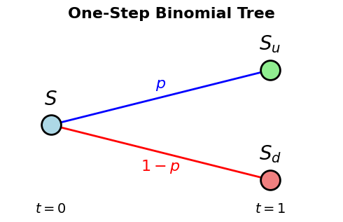
The simpliest option pricing model is the Binomial Option Pricing Model (BOPM)
BOPM Assumptions
We want to price an option on a stock trading at \(S\) currently
There are only two discrete times (one time step)
Today at \(t=0\),
Maturity of the option at \(t=1\)
At \(t=1\), the stock price can either go up to \(S_u\) or go down to \(S_d\) (two states)
Option payoff at \(t=1\) is \(C_u\) if the stock goes up and \(C_d\) if it goes down
If it is a call option then \(C_u = (S_u - K)^+\) and \(C_d = (S_d - K)^+\)
[20]:
# Single-step binomial tree visualization
import matplotlib.pyplot as plt
import matplotlib.patches as mpatches

fig, ax = plt.subplots(figsize=(5, 3))

# Node positions
t0_x, t0_y = 0, 0.5
t1_u_x, t1_u_y = 1, 0.75
t1_d_x, t1_d_y = 1, 0.25

# Draw edges (branches)
ax.plot([t0_x, t1_u_x], [t0_y, t1_u_y], 'b-', lw=2, label='Up move')
ax.plot([t0_x, t1_d_x], [t0_y, t1_d_y], 'r-', lw=2, label='Down move')

# Draw nodes
node_size = 400
ax.scatter([t0_x], [t0_y], s=node_size, c='lightblue', edgecolors='black', zorder=5, linewidths=2)
ax.scatter([t1_u_x], [t1_u_y], s=node_size, c='lightgreen', edgecolors='black', zorder=5, linewidths=2)
ax.scatter([t1_d_x], [t1_d_y], s=node_size, c='lightcoral', edgecolors='black', zorder=5, linewidths=2)

# Add labels
ax.text(t0_x, t0_y+0.12, r'$S$', fontsize=20, ha='center', va='center', fontweight='bold')
ax.text(t1_u_x, t1_u_y+0.12, r'$S_u$', fontsize=20, ha='center', va='center', fontweight='bold')
ax.text(t1_d_x, t1_d_y+0.12, r'$S_d$', fontsize=20, ha='center', va='center', fontweight='bold')

# Add probability labels on branches
ax.text(0.5, 0.65, r'$p$', fontsize=16, ha='center', va='bottom', color='blue', style='italic')
ax.text(0.5, 0.35, r'$1-p$', fontsize=16, ha='center', va='top', color='red', style='italic')

# Time labels
ax.text(t0_x, 0.15, r'$t=0$', fontsize=14, ha='center', va='top')
ax.text(t1_u_x, 0.15, r'$t=1$', fontsize=14, ha='center', va='top')

# Formatting
ax.set_xlim(-0.2, 1.3)
ax.set_ylim(0.2, 0.9)
ax.set_aspect('equal')
ax.axis('off')
ax.set_title('One-Step Binomial Tree', fontsize=16, fontweight='bold', pad=20)

plt.tight_layout()
plt.show()
BOPM No-Arbitrage Argument
We set up a portfolio so that, at \(t=1\), the portfolio value replicates the option in both states
By no-arbitrage argument, the option price at \(t=0\) should equals the portfolio value at \(t=0\)
The portfolio setup at \(t=0\):
Buy \(h\) share of the stock at \(S\)
Deposit \(B\) dollars into the money market account (MMA)
Initial portfolio value is \(hS+B\)
At \(t=1\) there are two states
Stock position value goes up to \(hS_u\) and cash in MMA grows into \(BM\) dollars
Stock position value goes down to \(hS_d\) and cash in MMA grows into \(BM\) dollars
To replicate the option payoff, set \begin{align*} hS_u + BM &= C_u\\ hS_d + BM &= C_d \end{align*}
Solve for \(h\) and \(B\) and find the initial portfolio value, which should equal the option price
BOPM
We have the system of equations written in matrix form \begin{align*} \begin{pmatrix} S_u & M\\ S_d & M \end{pmatrix} \begin{pmatrix} h \\ B \end{pmatrix} = \begin{pmatrix} C_u \\ C_d \end{pmatrix} \end{align*}
The solution is \begin{align*} \begin{pmatrix} h \\ B \end{pmatrix} = \frac{1}{M(S_u - S_d)} \begin{pmatrix} M & -M\\ -S_d & S_u \end{pmatrix} \begin{pmatrix} C_u \\ C_d \end{pmatrix} \end{align*}
The option price is \(hS + B\), or \begin{align*} \begin{pmatrix} S & 1 \end{pmatrix} \begin{pmatrix} h \\ B \end{pmatrix} &= \frac{1}{M(S_u - S_d)} \begin{pmatrix} S & 1 \end{pmatrix} \begin{pmatrix} M & -M\\ -S_d & S_u \end{pmatrix} \begin{pmatrix} C_u \\ C_d \end{pmatrix}\\ &= \frac{1}{M} \begin{pmatrix} \frac{SM - S_d}{S_u - S_d} & \frac{S_u - SM}{S_u - S_d} \end{pmatrix} \begin{pmatrix} C_u \\ C_d \end{pmatrix}\\ &= \frac{1}{M} \left( \frac{SM - S_d}{S_u - S_d} C_u + \frac{S_u - SM}{S_u - S_d} C_d \right) \end{align*}
BOPM Discussion
PV of the option at \(t=0\):
\[C = \frac{1}{M} \left( \frac{SM - S_d}{S_u - S_d} C_u + \frac{S_u - SM}{S_u - S_d} C_d \right),\]where \(1/M\) is the discount factor and
\[\frac{SM - S_d}{S_u - S_d} + \frac{S_u - SM}{S_u - S_d} = 1,\]which allows us to see \(C\) as a discounted expectation of possible option payoff
Weighted average with weights sum to 1 is an expectation
We write
\[\tilde p = \frac{SM - S_d}{S_u - S_d}, \qquad (1-\tilde p) = \frac{S_u - SM}{S_u - S_d},\]known as the risk neutral probability, different from the physical probability \((p, 1-p)\)
The precise statement is, \(C\) is a discounted expectation of possible option payoff under the risk neutral probability
BOPM Discussion (Cont.)
The physical probability \((p, 1-p)\) doesn’t go into option pricing
No matter how large \(p\) is (how likely the stock price will go up), the call option price doesn’t go up a bit in BOPM
Remember the option price we obtained is by a no-arbitrage argument. Quoting a different price will lead to an arbitrage opportunity
BOPM: Example
Consider an ATM call option in BOPM with \(S = K = 100\), \(K\) the strike price, and \(S_u = 105\), \(S_d = 95\), \(M=1.01\). Option payoff at \(t=1\) is \begin{align*} C_u &= (S_u - K)^+ = 5\\ C_d &= (S_d - K)^+ = 0 \end{align*}
PV of the option at \(t=0\) is \begin{align*} C &= \frac{1}{M} \left( \frac{SM - S_d}{S_u - S_d} C_u + \frac{S_u - SM}{S_u - S_d} C_d \right)\\ &= \frac{1}{1.01}\left( \frac{101 - 95}{105 - 95} \times 5 + \frac{105 - 101}{105 - 95} \times 0 \right) = \$ 2.970297 \end{align*}
BOPM: Example (Cont.)
One can compute the replicating portfolio as follows \begin{align*} \begin{pmatrix} h \\ B \end{pmatrix} &= \frac{1}{M(S_u - S_d)} \begin{pmatrix} M & -M\\ -S_d & S_u \end{pmatrix} \begin{pmatrix} C_u \\ C_d \end{pmatrix}\\ &= \frac{1}{1.01\times (105 - 95)} \begin{pmatrix} 1.01 & -1.01\\ -95 & 105 \end{pmatrix} \begin{pmatrix} 5 \\ 0 \end{pmatrix} = \begin{pmatrix} 0.5 \\ -47.0297 \end{pmatrix} \end{align*}
Buy \(0.5\) shares of the underlying and borrow \(\$47.0297\) in MMA at \(t=0\). The portfolio value at \(t=1\), in the cases the stock goes up and down, are \begin{align*} 0.5\times 105 - 47.0297\times 1.01 &= \$5,\\ 0.5\times 95 - 47.0297\times 1.01 &= \$0, \end{align*} respctively, which equal \(C_u\) and \(C_d\)
BOPM: Example (Cont..)
So far in the example, there is no physical probability \(p\) (because there is no need)
If an agent is confident the stock will go up (meaning the belief is the option price at \(t=1\) will be \(\$5\) with high probability \(p\)), and quotes \(C=\$4\) at today (\(t=0\)), how can you arbitrage?
Short sell the option to the agent to get \(\$4\) and spend \(\$2.970297\) to set up the replicating portfolio today. Your net cash inflow is \(4-2.970297 = \$1.029703\) at \(t=0\)
At \(t=1\), your obligation as an option writer (seller) is to pay the agent \(\$5\) if the stock goes up, and \(\$0\) if the stock goes down
But at \(t=1\), the replicating portfolio value is \(\$5\) if stock goes up and \(\$0\) if it goes down
In either case, you can liquidate the portfolio to fullfill your obligation
You are left with free cash inflow of \(\$1.029703\) at \(t=0\)
BOPM: Example (Cont…)
If the stock price did go up at \(t=1\) as expected by the agent, you pay the agent \(\$1\), as you sold the option at time \(t=0\) at the price \(\$4\) and buy it back at time \(t=1\) at the price \(C_u = \$5\)
But you still get to keep your risk free cash flow of \(\$1.029703\) at \(t=0\)
If you think this is a win-win situation as no one gets hurt, you are wrong
The agent could have made \(\$2\) by quoting the option at \(\$3\)
There is still room (\(3-2.970297 = \$0.029703\)) for arbitrage, and the market players will be happy to make the risk free profit
BOPM: Exercise
What’s the time zero PV of an ATM call option in BOPM with \(S = K = 100\), \(K\) the strike price, and \(S_u = 103\), \(S_d = 97\), \(M=1.01\)?
At \(t=0\), how many shares should you hold and how much money should you put in your MMA in order to set up a replicating portfolio?
Universal Option Pricing Formula
We’ve seen in BOPM that option price is a discounted expectation in the risk-neutral probability
This is true in general, regardless of the model (assumptions) used for the option pricing
Let \(X\) be any European payoff, a function of the underlying. Then the option price \(C\) is \begin{align*} C = M_0 \widetilde E[M_T^{-1} X] \end{align*}
An option pricing model specifies a distribution of the underlying (among other things) in the risk-neutral probability \(\widetilde P\)
Given the distribution, \(C\) is simply an integral
Change of Numeraire
The universal pricing formula \begin{align*} C = M_0 \widetilde E[M_T^{-1} X] \end{align*} is a special case of an even more general result
When we say \(S=\$100\) that means \(100\) USD, or \(100\) units of MMA
Any tradable asset can be used to denominate the underlying of the option
Examples are annuity and ZCB
“The underlying is trading at how many units of the annuity?”
The tradable asset used to denominate the underlying is known as the numeraire
Each numeraire is associated with a so-called equivalent martingle measure
The risk-neutral probability a special case of the equivalent martingle measure when using MMA as the numeraire
Let \(N_t\) be the numeraire used in option pricing, and the corresponding equivalent martingle measure is \(P^N\), then the time zero option price is \begin{align*} C &= N_0 E^N[N_T^{-1} X] \end{align*}
Change of Numeraire (Cont.)
The universal pricing formula \begin{align*} C = M_0 E^M[M_T^{-1} X] = N_0 E^N[N_T^{-1} X] \end{align*}
If you change a numeraire, you change the probability measure, and the distribution of the underlying
In fact, sometimes that’s the reaosn we change the numeraire: In the risk-neutral measure the distribution under some model is not known in closed form, but the distribution is known in closed form in a different measure so we can write the expectation as an integral
We will see example in SOFR caps and floors and swaptions pricing
An option pricing model can also specify a distribution of the underlying (among other things) in any equivalent martingle measure
SOFR Swaption
A swaption gives the holder the right, but not the obligation, to enter into a swap with a predetermined fixed rate (the strike) in the future
A 1y10y payer swaption with strike \(4\%\) is the right to enter into a 10y payer swap, with fixed rate \(4\%\), 1 year from now
1y is the expiry, or maturity, of the swaption
10y is the tenor
The end date of a 1y10y swaption will be 11y from now
Both parties are looking at the forward starting 10y swap with fixed rate \(4\%\), which starts 1y from now
If, at expiry, the spot starting 10y swap rate is higher than \(4\%\), say it’s \(5\%\), then the holder will exercise the option and enter into the payer swap
The holder will recieve floating coupons and pay \(4\%\) fixed coupons, at the end of every year, for the following 10 years
The holder then can enter into a spot starting receiver swap at \(5\%\), receiving \(5\%\) fixed coupons while paying floating
The net cash inflow is a \(1\%\) fixed coupon at the end of every year for 10y
If, at expiry, the spot starting 10y swap rate is lower than \(4\%\), then the option expires worthless
Forward Starting Swap PV Clean Form (Review)
Consider a tenor structure
\[T_0 < T_1 < T_2 < \cdots < T_N, \qquad \tau_n = T_{n+1} - T_n\quad \forall n=0, 1, 2, \ldots, N-1,\]where \(\tau_n\) is fixed to be 1Y
The time-\(t\) PV of an \(N\)-year-long forward starting payer swap with fixed rate \(K\) is \begin{align*} &\sum_{n=0}^{N-1}\left(\tau_n P(t, T_{n+1})L(t, T_n, T_{n+1}) - \tau_n P(t, T_{n+1})K\right)\\ =& \left(\sum_{n=0}^{N-1}\tau_n P(t, T_{n+1})\right)\left(\frac{\sum_{n=0}^{N-1}\tau_n P(t, T_{n+1})L(t, T_n, T_{n+1})}{\sum_{n=0}^{N-1}\tau_n P(t, T_{n+1})} - K\right) \\\\ =& A(t)(S(t) - K) \end{align*}
Here \(K\) is the strike \(4\%\) in the previous example
The forward starting swap rate \(S(t)\) fixes at \(S(T_0)\) to become the spot starting swap rate (\(5\%\) in the previous example)
Swaption Payoff
As explained earlier, if \(S(T_0) > K\) then the holder will exercise the payer swaption and if not, the option expires worthless
If \(S(T_0) > K\), the holder will enter into the swap with a nonzero initial NPV
\[A(T_0)(S(T_0)-K)\]Thus the payer swaption payoff is
\[X = A(T_0)(S(T_0)-K)^+\]which is a function of the underlying \(S(T_0)\)
This payoff makes annuity \(A(t)\) the natural choice of the numeraire for swaption pricing
Swaption Pricing
Payer swaption payoff
\[X = A(T_0)(S(T_0)-K)^+\]Payer swaption PV at time \(t\) \begin{align*} C &= A(0)E^A[A(T_0)^{-1} X]\\ &= A(0)E^A[(S(T_0)-K)^+] \end{align*}
From here we will need to specify a model, including a distribution of \(S(T_0)\)
The simpliest choice is the normal distribution \(N(0, \sigma^2T_0)\), which is the Black Normal model
SOFR Caps and Floors
Consider a tenor structure
\[T_0 < T_1 < T_2 < \cdots < T_N, \qquad \tau_n = T_{n+1} - T_n\quad \forall n=0, 1, 2, \ldots, N-1,\]where \(\tau_n\) is now fixed to be 3M
A 3M SOFR cap with strike \(K\) pays the buyer a series of cash flows
\[\tau_n(L(T_{n+1}, T_{n}, T_{n+1}) - K)^+ \quad\text{ at }\quad T_{n+1}, \quad \forall n=0, 1, 2, \ldots, N-1,\]where \(L(T_{n+1}, T_{n}, T_{n+1})\) is the SOFR term rate
Similarly, a 3M SOFR floor with strike \(K\) pays the buyer a series of cash flows
\[\tau_n(K - L(T_{n+1}, T_{n}, T_{n+1}))^+ \quad\text{ at }\quad T_{n+1} \quad \forall n=0, 1, 2, \ldots, N-1\]
Why the Name
Imagine you have liabilities to pay floating coupon \(\tau_n L(T_{n+1}, T_n, T_{n+1})\) every quarter (3M)
The payment to be made is unknown until the end of every coupon period, \(T_{n+1}\)
If you buy a cap with \(K = 6\%\), when the term rate fixes to be lower than \(6\%\), from the cap you recieve nothing:
\[\tau_n(L(T_{n+1}, T_n, T_{n+1}) - K)^+ = 0\]Given the liability, you will pay a lower than \(6\%\) coupon rate: \(\tau_n L(T_{n+1}, T_n, T_{n+1})\)
But if the forward rate fixed to be larger than \(6\%\), from the cap you recieve
\[\tau_n(L(T_{n+1}, T_n, T_{n+1}) - K)^+ = \tau_n(L(T_{n+1}, T_n, T_{n+1}) - K)\]Given the liability, you still pay a the coupon \(\tau_n L(T_{n+1}, T_n, T_{n+1})\)
Overall you pay \(\tau_n K\) which is at \(6\%\) annual coupon rate
If you buy a \(6\%\) cap, your payment is capped at \(6\%\) annual rate